require(igraph)
g <- graph(c(1,2), n=2, dir=FALSE)
plot(g, vertex.color="skyblue2",vertex.label.family="Helvetica")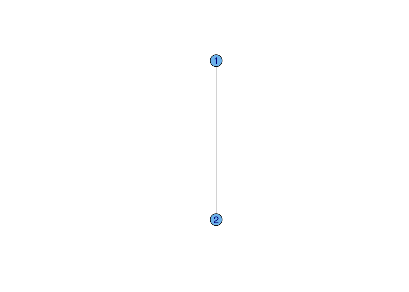
A graph is simply a collection of vertices (or nodes) and edges (or ties). We can denote this \(\mathcal{G}(V,E)\), where \(V\) is the vertex set and \(E\) is the edge set. The vertices of the graph represent the actors in the social system. These are usually individual people, but they could be households, geographical localities, institutions, or other social entities. The edges of the graph represent the relations between these entities (e.g., “is friends with” or “has sexual intercourse with” or “sends money to”). These edges can be directed (e.g., “sends money to”) or undirected (e.g., “within 2 meters of”). When the relations that define the graph are directional, we have a directed graph or digraph. The edges in a graph connect unordered pairs of vertices and are sometimes called lines. The edges in a digraph connect ordered pairs of vertices and are sometimes called arcs. Graphs (and digraphs) can be binary (i.e., presence/absence of a relationship) or valued (e.g., “groomed five times in the observation period”, “sent $100”). When an edge connects to a vertex, it is said to be incident to that vertex. The number of edges that are incident to vertex \(v_i\) is the degree of \(v_i\) and the collection of all degrees of a graph is known as the degree distribution. A vertex with degree zero is an isolate. The number of vertices in a graph is the order of the graph.
A graph (with no self-loops) with \(n\) vertices has \({n \choose 2} = n(n-1)/2\) possible unordered pairs. This number (which increases very rapidly with \(n\)) is important for defining the density of a graph, which is the fraction of all possible relations that actually exist in a network.
The most basic non-trivial graph is a connected dyad. Note that a dyad is simply a pair of vertices, connected or not. This graph has two vertices and a single edge. We can create and visualize this graph using igraph.
require(igraph)
g <- graph(c(1,2), n=2, dir=FALSE)
plot(g, vertex.color="skyblue2",vertex.label.family="Helvetica")
The call to the function graph() takes three arguments in this case. First, we enumerate the edges by listing the pairs of vertices which are connected. In this graph, there is only a single edge, so our first argument only contains one pair. Second, we define the size of our graph. This simple graph has only two vertices, so n=2. Third, the default graph type is directed, so to create an undirected graph, we need to specify dir=FALSE. The function graph() creates a graph object which, like any R object, is associated with a number of methods. When we plot a graph object, the plotting method used is plot.igraph(). There are a number of features (or perhaps peculiarities) of the defaults of plot.igraph(). First, is the vertex color. It’s not hideous but it’s not an obvious choice for a default color either. Second, the default font label style is Roman, which can make the labels look cluttered. I typically change to a sens-serif font using the argument vertex.label.family="Helvetica". Third, the layout will not necessarily make sense to you as a human viewer of the graph and will typically change each time you call plot.igraph(). Fortunately, igraph has a number of excellent tools for assisting with graph layout.
A very handy utility for assisting with the layout of small graphs is tkplot(). Calling tkplot() will open an X11 window (the specifics of which might vary depending on your operating system). When your graph opens in this window, you will be able to move vertices around until you have a layout that you like. You then use the function tk_coords(tkp.id) (where tkp.id is the window number of your tkplot) to get the coordinates of your vertices. Showing how to use tkplot() in a document such as this is difficult, since it is an intrinsically interactive exercise. However, we can see how to layout a small graph once you have acquired the coordinates from tk_coords().
# generate a triangle
g <- graph( c(1,2, 2,3, 1,3), n=3, dir=FALSE)
### do some stuff with tkplot() and get coords which we call tri.coords
tri.coords <- matrix( c(228,416, 436,0, 20,0), nr=3, nc=2, byrow=TRUE)
par(mfrow=c(1,2))
plot(g, vertex.color="skyblue2",vertex.label.family="Helvetica")
plot(g, layout=tri.coords, vertex.color="skyblue2",vertex.label.family="Helvetica")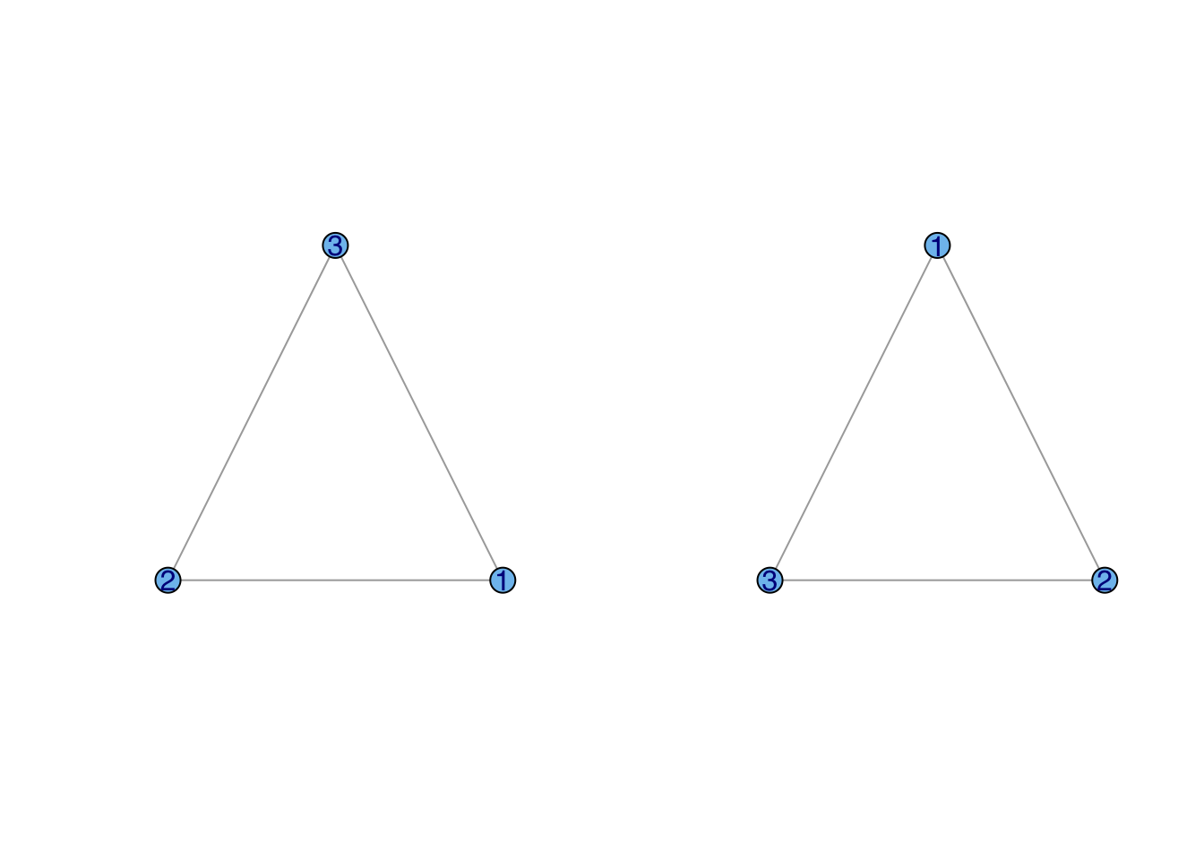
We can represent the relationships of our social network using a matrix. A matrix is simply a rectangular array of numbers with (n) rows and \(k\) columns. It is conventional to denote matrices mathematically using capital letters and boldface, such as \(\mathbf{A}\). We indicate the \(ij\)th element (i.e., the element corresponding to row \(i\) and column \(j\)) of \(\mathbf{A}\) as \(a_{ij}\). A sociomatrix or adjacency matrix is a square matrix (i.e., \(n \times n\), where \(n\) is the number of vertices in the network). It is typically binary, with \(a_{ij}=1\) if individuals \(i\) and \(j\) share an edge and \(a_{ij}=0\) otherwise. The sociomatrix corresponding to our triangle is
\[\begin{equation} \mathbf{A} = \left[ \begin{array}{cccc} 0 & 1 & 1 \\ 1 & 0 & 1 \\ 1 & 1 & 0 \end{array} \right]. \end{equation}\]
By convention, the diagonal elements of a sociomatrix are all zero (i.e., self-loops are not allowed). Sociomatrix \(\mathbf{A}\) in the equation above is symmetric (\(a_{ij} = a_{ji}\)) because the graph is undirected. For a digraph, the upper triangle (i.e., matrix elements above the diagonal) of the sociomatrix will generally be different than the lower triangle.
A <- matrix( c(0,1,1, 1,0,1, 1,1,0), nrow=3, ncol=3, byrow=TRUE)
g <- graph_from_adjacency_matrix(A, mode="undirected", diag=FALSE)
plot(g, layout=tri.coords, vertex.color="skyblue2",vertex.label.family="Helvetica")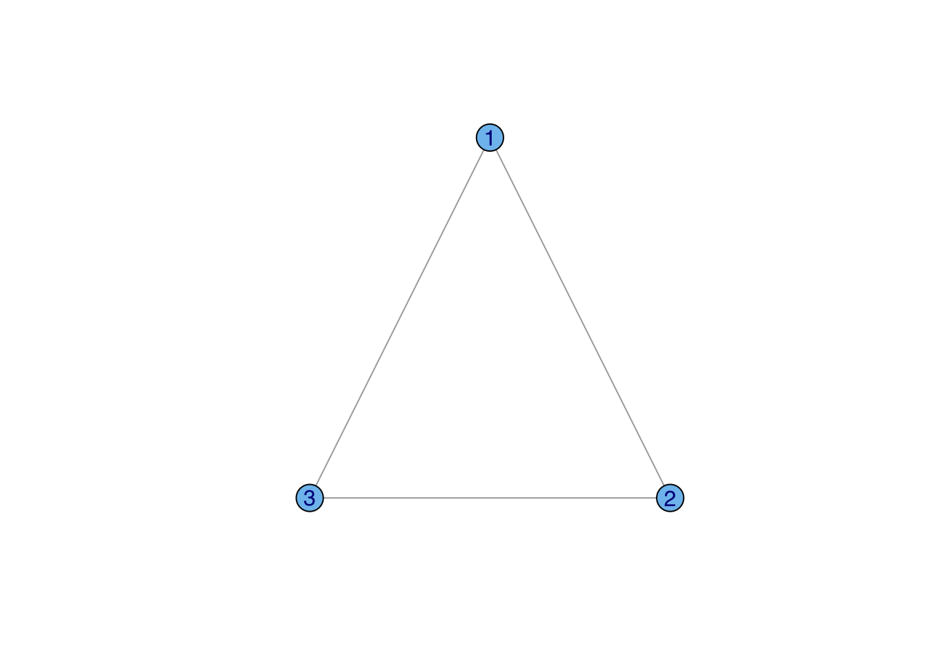
We can make a cyclical triangle too:
A1 <- matrix( c(0,1,0, 0,0,1, 1,0,0), nrow=3, ncol=3, byrow=TRUE)
g1 <- graph_from_adjacency_matrix(A1, mode="directed", diag=FALSE)
plot(g1, layout=tri.coords, vertex.color="skyblue2",vertex.label.family="Helvetica")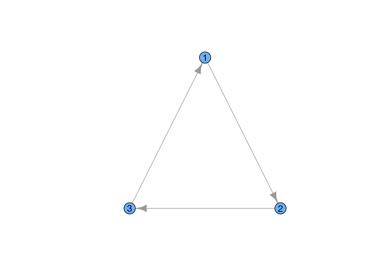
Note that we can keep recycling the same layout since we still have a triangle, even if its structure is different.
Most graphs are more complex than a single edge or triangle. This means that we need to be able to read data files into igraph (or whatever library we’re using, such as sna). We can easily read a sociomatrix directly into R and then import it into igraph. A sociomatrix from Kapferer’s classic (1972) study of social relations in a tailor shop in colonial North Rhodesia (now Zambia) describes the “instrumental” social interactions between 39 actors before organizing for an unsuccessful strike. We first read the matrix file into R while simultaneously converting it to a matrix (R will otherwise treat it as a data frame). We then import the sociomatrix into igraph and plot the results.
A <- as.matrix(read.table("data/kapferer-tailorshop1.txt",
                          header=TRUE, row.names=1))
G <- graph_from_adjacency_matrix(A, mode="undirected", diag=FALSE)
plot(G, vertex.color="skyblue2", vertex.label.family="Helvetica")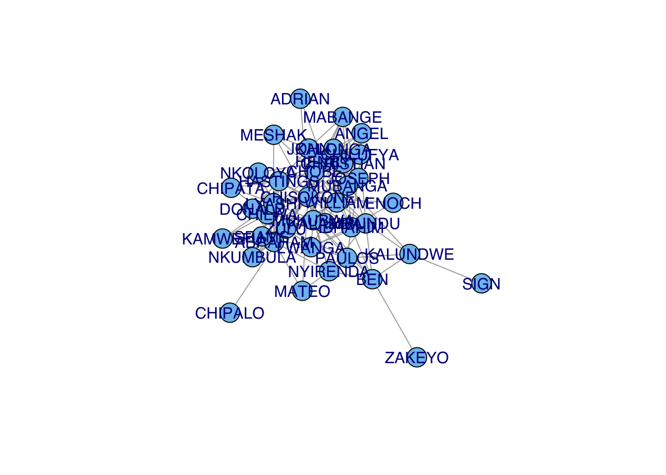
Note that the matrix contains row/column names (i.e., the pseudonyms for the 39 actors). These names are preserved as a vertex attribute in the igraph network object. When we plot, by default, these names are printed along with the vertices. Sometimes, when we have vertex names, it looks better to supress the vertices.
plot(G,vertex.shape="none", vertex.label.cex=0.75, edge.color=grey(0.85),vertex.label.family="Helvetica")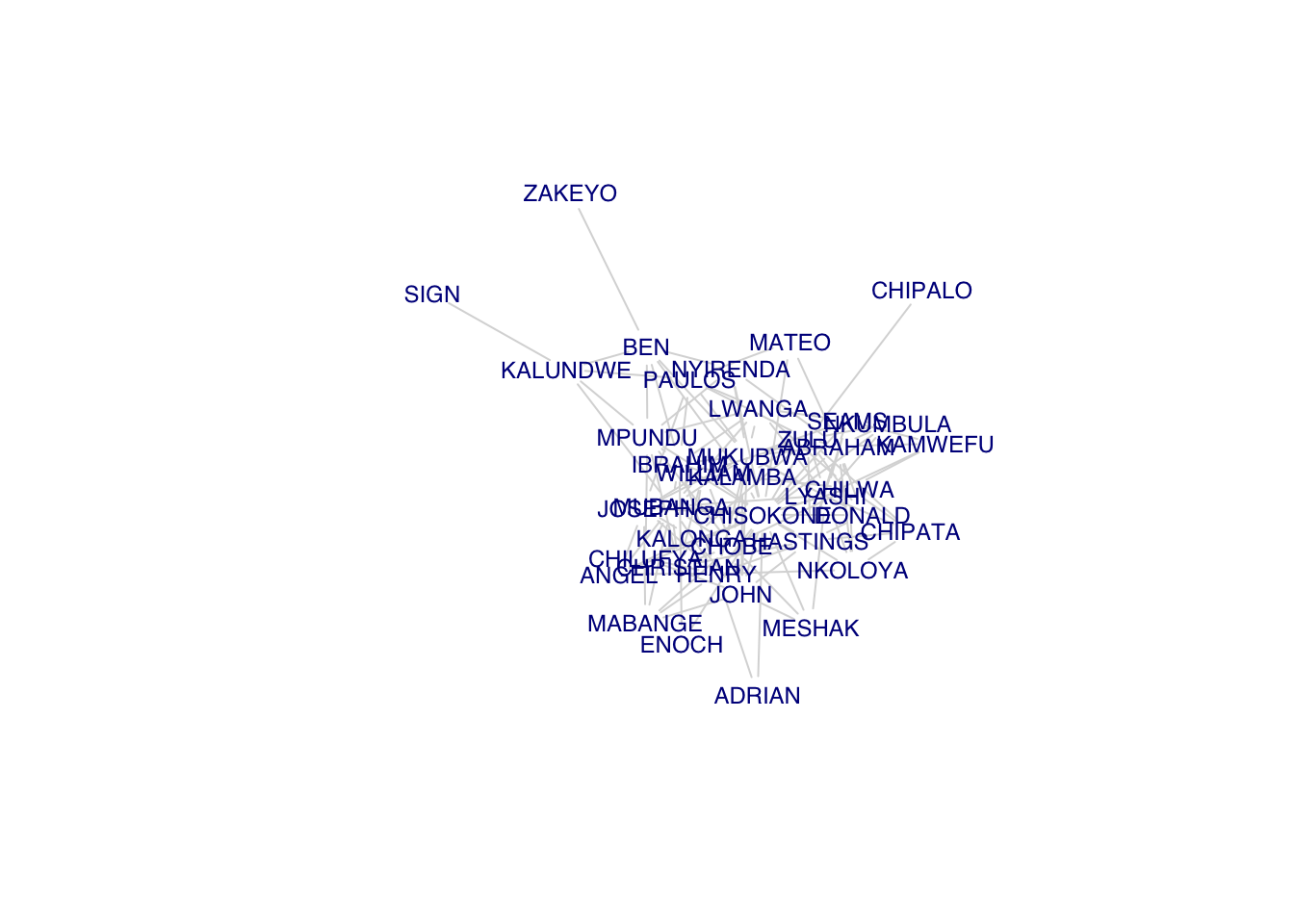
In addition to supressing the vertices, we’ve made the text size a bit smaller vertex.label.cex=0.75 and made the edge color lighter to make the labels more readable, edge.color=grey(0.85).
Typically, we have to play around a lot with the layout. The tailor shop data show a common frustration. Note the Chipalo, Sign and Zakeyo are relatively isolated, while most everyone is is highly connected
require(igraph)
sort(degree(G))
CHIPALO SIGN ZAKEYO ENOCH ADRIAN MATEO KAMWEFU MESHAK
1 1 1 2 2 3 4 4
NKUMBULA CHIPATA NYIRENDA KALUNDWE MABANGE DONALD NKOLOYA ANGEL
5 5 5 5 5 6 6 6
PAULOS BEN LWANGA KALAMBA CHRISTIAN SEAMS CHILWA MPUNDU
7 7 8 8 8 9 9 9
JOHN CHILUFYA HASTINGS JOSEPH WILLIAM CHOBE KALONGA IBRAHIM
9 9 10 10 10 10 10 11
ABRAHAM ZULU HENRY MUBANGA LYASHI MUKUBWA CHISOKONE
13 14 14 14 15 17 24 ego(G,order=1,nodes=c(10,20,22))[[1]]
+ 2/39 vertices, named, from 10a426e:
[1] CHIPALO ZULU
[[2]]
+ 2/39 vertices, named, from 10a426e:
[1] SIGN KALUNDWE
[[3]]
+ 2/39 vertices, named, from 10a426e:
[1] ZAKEYO BEN ## not that enlightening
ego(G,order=2,nodes=c(10,20,22))[[1]]
+ 15/39 vertices, named, from 10a426e:
[1] CHIPALO ZULU NKUMBULA ABRAHAM SEAMS CHIPATA DONALD
[8] LYASHI HASTINGS CHISOKONE PAULOS MUKUBWA KALAMBA WILLIAM
[15] KALONGA
[[2]]
+ 6/39 vertices, named, from 10a426e:
[1] SIGN KALUNDWE PAULOS BEN MPUNDU MUBANGA
[[3]]
+ 8/39 vertices, named, from 10a426e:
[1] ZAKEYO BEN NYIRENDA MUKUBWA KALAMBA IBRAHIM KALUNDWE MPUNDU By using the function ego() we can see what the neighborhood around these near-isolates looks like. When we look at the first-order ego networks, they are all the same (ego plus their one alter). However, Chipalo is plotted closer to the cohesive core than either Sign or Zakeyo. Why is that? When we investigate the second-order ego network, we see that Chipalo’s single alter, Zulu, is among the most connected individuals in the tailor shop, with a degree of \(k=14\). This means that Chipalo is closer to the core than the others, so he is less peripheral to the overall layout.
Now that we have a non-trivial graph, we can talk some more about graph properties. A subgraph is a graph \(\mathcal{G}^{\prime}\) where all the vertices and edges are also in graph \(\mathcal{G}\). Subgraphs can be generated by selecting either vertices or the edges from \(\mathcal{G}\). We commonly want to filter subgraphs that we think correspond to some sociological grouping. A very active area of research in the analysis of social networks is the field of community detection. We will talk about community detection in a different set of notes. For now, just think of it as a way of defining a set of vertices for a subgraph of G.
fg <- cluster_fast_greedy(G)
subg1 <- induced_subgraph(G, which(membership(fg)==4))
summary(subg1)
IGRAPH 16fe2de UN-- 12 33 --
+ attr: name (v/c)plot(subg1,vertex.shape="none", vertex.label.cex=0.75,
edge.color=grey(0.85),vertex.label.family="Helvetica")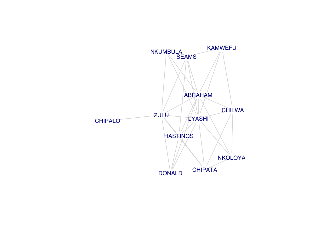
The subgraph subg1 is connected, which means that there is a path between all the vertices of subg1. A path is a walk with no repeated vertex, where a walk is simply an alternating sequence of vertices and edges. When there is a path between two vertices \(v_1\) and \(v_2\), we say that \(v_1\) is reachable from \(v_2\) and vice-versa. This means that all vertices within a connected subgraph are reachable from all others.
Suppose we combine two of the detected communities (call that subg2) and then remove a few edges from this new subgraph.
subg2 <- induced_subgraph(G, which(membership(fg)==4 | membership(fg)==1))
## MATEO -- ABRAHAN: 9
## PAULOS -- ZULU: 39
## PAULOS -- LWANGA: 40
subg3 <- delete_edges(subg2, c(9, 39, 40))
par(mfrow=c(1,2))
plot(subg2, vertex.shape="none", vertex.label.cex=0.5, edge.color=grey(0.85),
     vertex.label.family="Helvetica")
plot(subg3, vertex.shape="none", vertex.label.cex=0.5, edge.color=grey(0.85),
     vertex.label.family="Helvetica")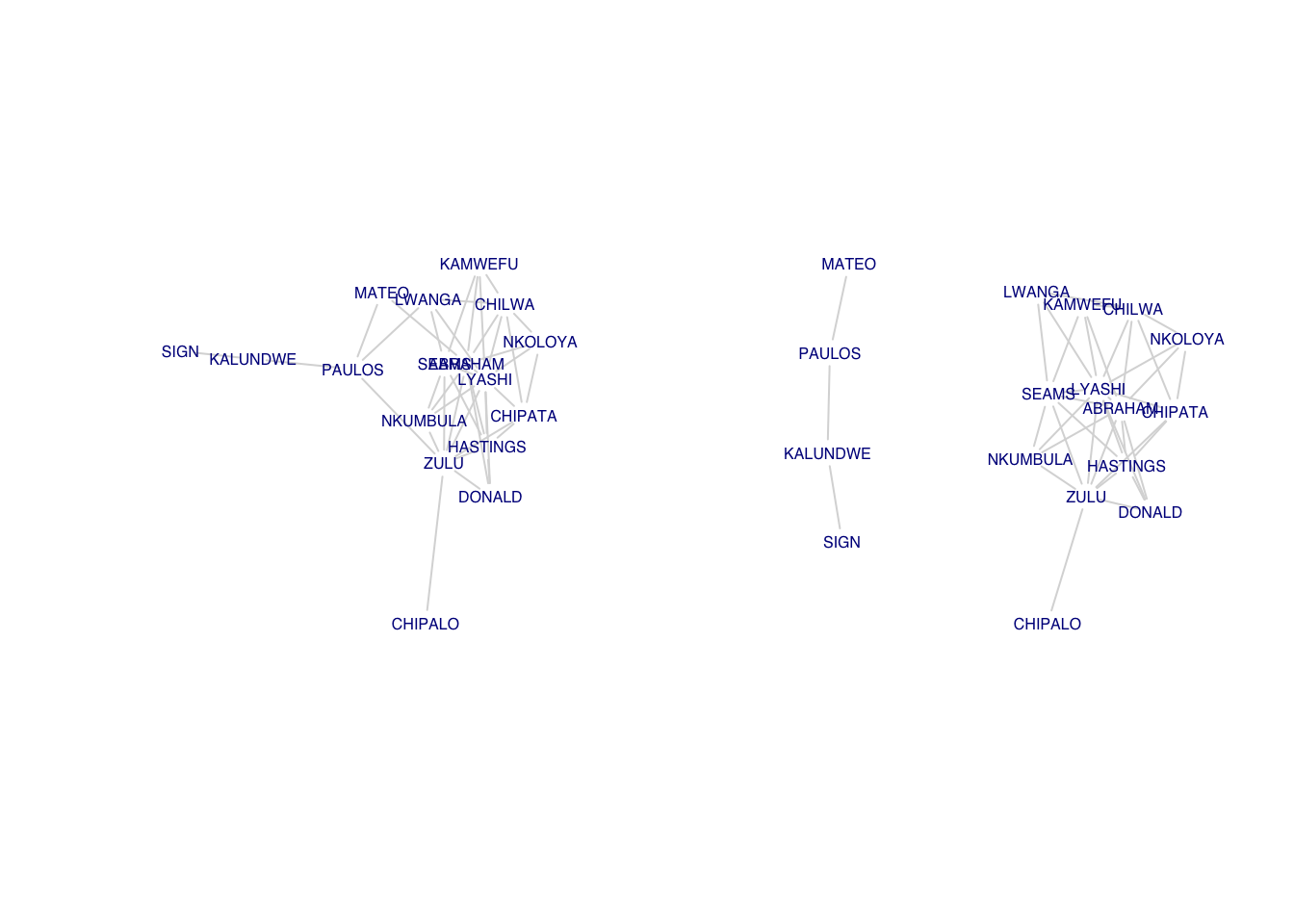
By removing three edges (Mateo-Abraham, Paulos-Zulu, Paulos-Lwanga) in our subgraph, we create two distinct components. A component is a maximally connected subgraph of a graph. In graph theory the property of maximality means that a subgraph \(\mathcal{G}^{\prime}\) is maximal for some property when the property holds for the subgraph but does not hold when additional vertices and incident edges are added. If we were to include a vertex from one of our two subgraphs of subg3 in the other, the subgraph would no longer be a subcomponent (since that vertex would have no incident edges to the subgraph so there would be no path between it and the other vertices in the subgraph). One cannot traverse a path from, say, Kalundwe to Nkumbula.
While the subgraph containing Sign, Kalundwe, Paulos, and Matteo, (call it \(G ^{\prime}_2\)) is maximally connected, this doesn’t mean that all members of \(G ^{\prime}_2\) are directly connected to each other – it only means that there is a path between each of its members. If every vertex in a subgraph is connected to every other vertex in that subgraph, the subgraph is known as a clique. A graph in which every vertex is adjacent to every other vertex is also known as a complete graph. What makes a clique a clique is that it is a complete graph that is a subgraph of some larger graph. Cliques or near-cliques play an important role in network clustering and community detection.
We can generate and plot a complete or “full” graph of rank five:
plot(make_full_graph(5), vertex.color="skyblue2")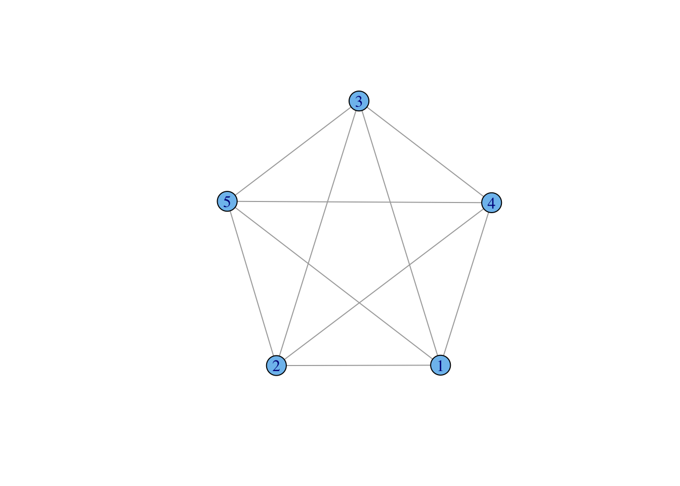
Complete graphs become particularly important when we discuss the estimation of regression models for social networks.
The degree of a vertex, which we can denote \(k\), is simply the number of edges incident to that vertex. For example, in the following figure, the degree of the light blue vertex is four.
g <- make_graph( c(1,2, 1,3, 1,4, 1,5), n=5, dir=FALSE )
mki <- c("skyblue2",rep("white",4))
lay <- matrix(c(0,0, 1,0, 0,1, -1,0, 0,-1),nr=5,nc=2,byrow = TRUE)
vf <- c("black", rep("white",4))
plot(g, vertex.label=NA, vertex.color=mki, vertex.frame.color=vf, edge.width=3, layout=lay)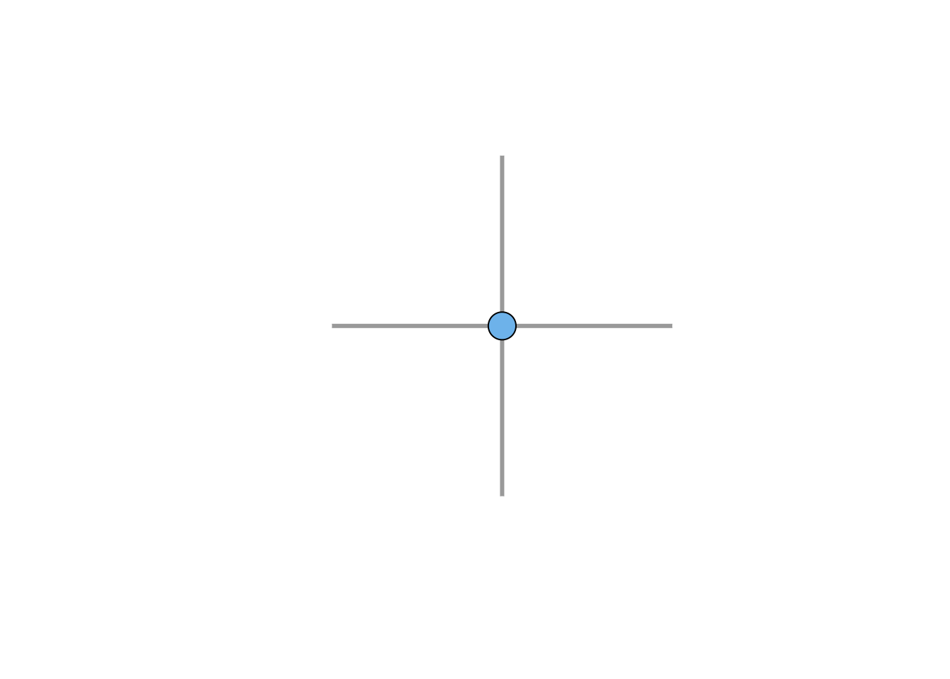
Degree is always calculated with respect to a single relation so that if you have a multiplex network (e.g., economic exchange and voluntary association co-membership), each vertex will have multiple degrees. If the graph is directed, then we define in-degree as the number of incoming directed edges incident to a vertex and the out-degree as the number of outgoing directed edges incident to a vertex.
The degree distribution of a graph is the aggregate of the individal degrees of the vertices of a graph. Degree distributions are very important for a number of features of interest in networks.
degree(G) KAMWEFU NKUMBULA ABRAHAM SEAMS CHIPATA DONALD NKOLOYA MATEO
4 5 13 9 5 6 6 3
CHILWA CHIPALO LYASHI ZULU HASTINGS LWANGA NYIRENDA CHISOKONE
9 1 15 14 10 8 5 24
ENOCH PAULOS MUKUBWA SIGN KALAMBA ZAKEYO BEN IBRAHIM
2 7 17 1 8 1 7 11
MESHAK ADRIAN KALUNDWE MPUNDU JOHN JOSEPH WILLIAM HENRY
4 2 5 9 9 10 10 14
CHOBE MUBANGA CHRISTIAN KALONGA ANGEL CHILUFYA MABANGE
10 14 8 10 6 9 5 Many networks reveal a highly-skewed degree distribution. Such skewed degree distributions can connect otherwise sparse networks and have been implicated, for example, in the persistence of infectious diseases in networks where the average behavior would otherwise lead to the extinction of the infection (May and Lloyd 2001). While many networks are indeed quite skewed, both the extent and the ubiquity of this phenomenon have been rather over-stated in the general networks literature Jones and Handcock (2003a) and many human social networks (especially face-to-face relationships that are not technologically mediated) are not remarkably skewed at all (Salathé et al. 2010).
It is conventional in much of the networks literature to plot degree distributions as the complement of the cumulative distribution function (a.k.a., the survivor function) on semi-logarithmic axes. This convention arose because a linear plot is suggestive of a power-law degree distribution and there has been substantial interest in power-laws in network phenomena. A much more robust plot is simply as a histogram, which will better reveal the probability mass function of the degree distribution. Note that using semi-logarithmic axes precludes the inclusion of degree \(k=0\), since the logarithm of zero is undefined. Vertices of degree zero, known as isolates are often very important in and of themselves and can be diagnostic of social process, so a plot that precludes their inclusion is highly problematic.
#g <- erdos.renyi.game(1000, 1/500) #old syntax!
g <- sample_gnp(1000,1/500)
dd <- degree_distribution(g)
lendd <- length(dd)
plot((1:lendd)-1,dd, type="h", lwd=20, lend=2, col="blue",
     xlab="Degree (k)", ylab="Probability(K=k)")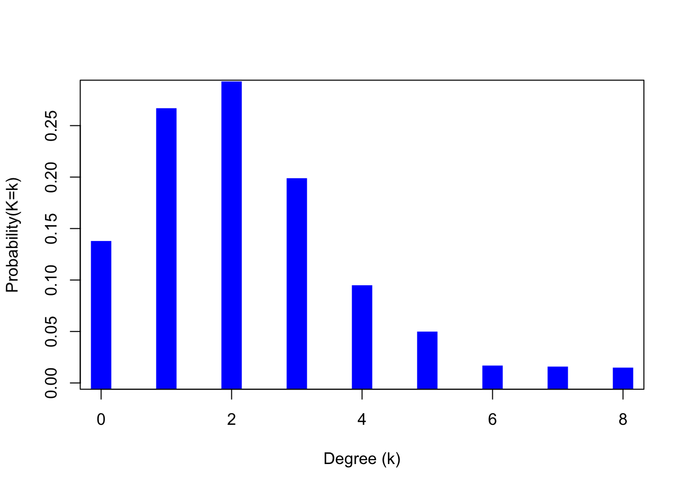
A geodesic is the shortest path between two vertices. Geodesics are important for centrality and network flow discussed in a later set of notes. The largest geodesic of a graph is known as the diameter of the graph. We can find the diameter for the Kapferer tailor shop network. There are only 39 actors in this network, and it is pretty densly connected, so the diameter is not huge (\(d=4\)). In fact, there are 54 geodesics of length four.
d <- get_diameter(G)
E(G)$color <- "SkyBlue2"
E(G)$width <- 1
E(G, path=d)$color <- "red"
E(G, path=d)$width <- 2
V(G)$labelcolor <- V(G)$color  <- "blue"
V(G)[d]$labelcolor <- V(G)[d]$color <- "red"
plot(G, vertex.shape="none", vertex.label.cex=0.5,
     edge.color=E(G)$color, edge.width=E(G)$width,
     vertex.label.color=V(G)$labelcolor,
     vertex.size=3)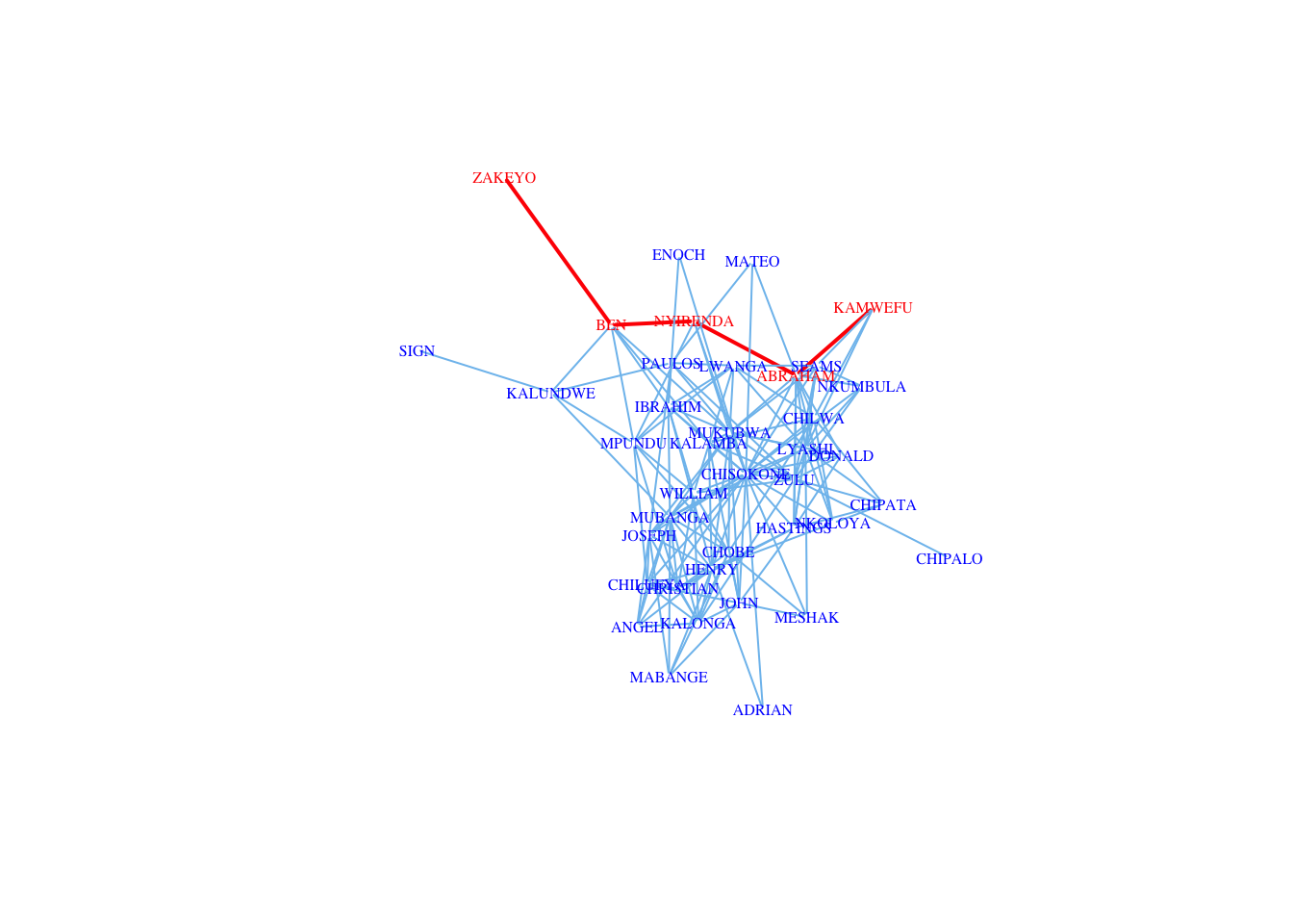
There are many, many formats for relational data. Probably the most universal and simplest is known as a edgelist. An edgelist is simply a two-column matrix in which each row represents a (possibly directed) edge between the vertex listed in first column and the second column. Note that this is essentially what we passed to the graph() function above.
We are often interested in evaluating how an observed social network differs from some theoretical network. To do this, it is useful to count various structures and compare the counts to known null models. Understanding these counts will eventually serve an important role in developing regression-like models for network inference. An important concept for dealing with triads (and other basic network structures) is isomorphism. Two graphs are said to be isomorphic if we cannot tell the difference between them when the vertex labels are removed. This is similar to the concept, which is critical in Bayesian statistics, of exchangeability.
A dyad is simply an unordered pair of vertices in a graph. As we have discussed previously, there are \({n \choose 2} = n(n-1)/2\) dyads in a graph of size \(n\).
In a directed graph, there are four different types of relations between vertices \(i\) and \(j\): \(i \rightarrow j\), \(i \leftarrow j\), \(i \leftrightarrow j\) and \(i~~j\).
g <- graph( c( 1,2, 3,4, 5,6, 6,5), n=8)
ccc <- cbind(c(300, 100, 100, 300, 100, 300, 100, 300),
             c(300, 300, 230, 230, 160, 160, 90, 90))
plot(g, layout=ccc, vertex.color=grey(0.75), vertex.label.family="Helvetica")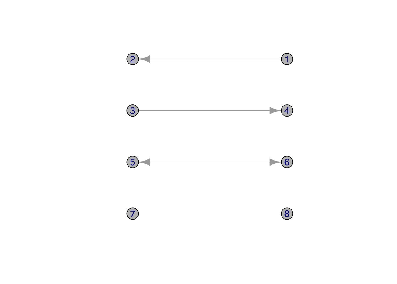
Note that \(i \rightarrow j\), \(i \leftarrow j\) are isomorphic.
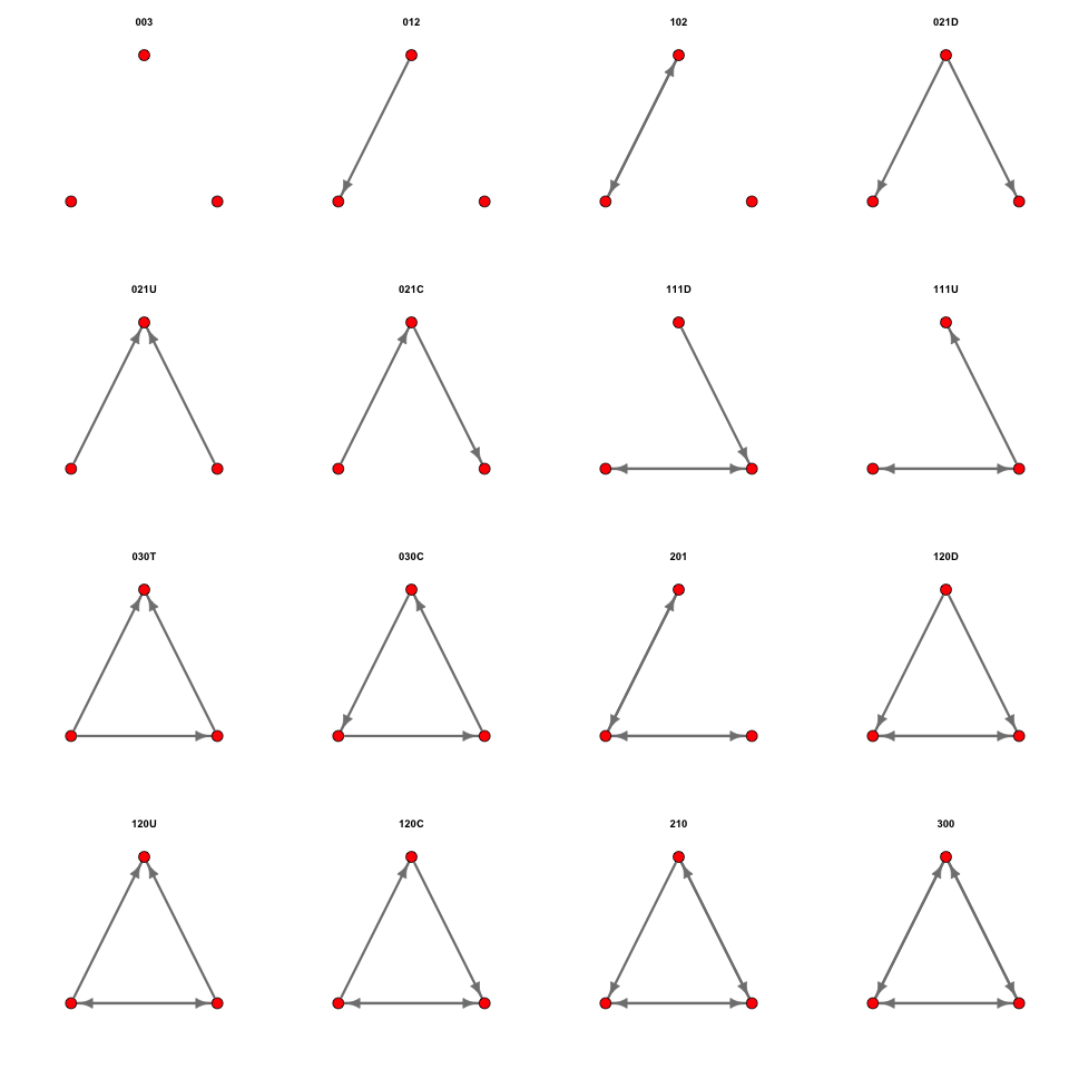
There is a conventional nomenclature for triads, following the pathbreaking paper by Davis and Leinhardt (1972). There are sixteen distinct triads:
| Triad | Edges |
|---|---|
| 003 | \(A,B,C\) |
| 012 | \(A \rightarrow B, C\) |
| 102 | \(A \leftrightarrow B, C\) |
| 021D | \(A \leftarrow B \rightarrow C\) |
| 021U | \(A \rightarrow B \leftarrow C\) |
| 021C | \(A \rightarrow B \rightarrow C\) |
| 111D | \(A \leftrightarrow B \leftarrow C\) |
| 111U | \(A \leftrightarrow B \rightarrow C\) |
| 030T | \(A \rightarrow B \leftarrow C, A \rightarrow C\) |
| 030C | \(A \leftarrow B \leftarrow C, A \rightarrow C\) |
| 201 | \(A \leftrightarrow B \leftrightarrow C\) |
| 120D | \(A \leftarrow B \rightarrow C, A \leftrightarrow C\) |
| 120U | \(A \rightarrow B \leftarrow C, A \leftrightarrow C\) |
| 120C | \(A \rightarrow B \rightarrow C, A \leftrightarrow C\) |
| 210 | \(A \rightarrow B \leftrightarrow C, A \leftrightarrow C\) |
| 300 | \(A \leftrightarrow B \leftrightarrow C, A \leftrightarrow C\) |
The table provides notation for the sixteen triads. The first number is the number of mutual dyads, the second is the number of asymmetric dyads, and the third is the number of null dyads in the triad. The letters stand for Up, Down, Cyclical, and Transitive. For example, 030T has zero mutual, three asymmetric, and zero null dyads and is transitive, whereas 030C has zero mutual, three asymmetric, and zero null dyads and is cyclical.
We can use the igraph command triad_census() to perform a triad census. The output is the count of the number of triads using the Davis and Leinhardt (1972) categorization, in the order of the table above.
g <- sample_gnm(15, 45, directed = TRUE)
plot(g,edge.arrow.width=0.5, vertex.color="skyblue2",
     vertex.label.family="Helvetica")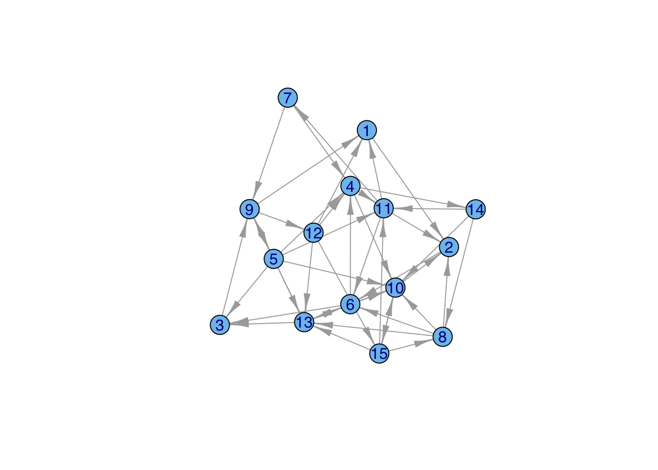
triad_census(g) [1] 93 192 12 25 30 58 12 6 15 4 1 1 2 4 0 0Transitivity implies dominance whereas cyclicity implies exchange. Transitivity implies dominance whereas cyclicity implies exchange. A linear hierarchy means that all triads must be transitive (030T) (Chase 1974). There’s an interesting parallel to expected utility theory here. Debreu representation theorem showed that a valid representation of (ordinal) utility must be complete and transitive. This yields a linear ordering of preferences.
## define triads
DD <- graph( c(3,1, 3,2), n=3, directed=TRUE)
DS <- graph( c(3,1, 2,1), n=3, directed=TRUE)
BDID <- graph( c(3,1, 2,3), n=3, directed=TRUE)
ISDB <- graph( c(3,1, 1,2), n=3, directed=TRUE)
labs <- c("B","C","A")
Linear dominance hierarchies are common in animal behavior. A linear dominance hierarchy implies that all triples in the network are of the 030T form. What gives rise to this? Chase (1974) noted that there are two standard explanations for linear dominance hierarchies: (1) the “tournament model” and (2) the “correlation model.” In the tournament model, individual dyads within a group pair off to establish dominance based on intrinsic qualities such as strength, aggressiveness or the size of weapons (e.g., canines, antlers). The overall dominance hierarchy is formed after an exhaustive “round-robin tournament” establishes all pairwise dominance interactions. In contrast, the correlation model proposes that a correlation exists between traits that predict dominance and the actual dominance interactions of the animals (e.g., antler size in red deer). Dominance hierarchies arise by animals sorting themselves along the dimension of this trait (which may be a composite).
Chase notes that these models, while intuitively appealing, are implausible. To yield a linear dominance hierarchy, the probabilities of victory in pairwise interactions or the strength of the correlation between the trait and actual dominance would have to be unrealistically high. Chase (1974: 378) writes that “extreme probability distributions are required to predict a strong hierarchy from a tournament no matter what the species of animal, the method of pairwise competition, or the individual traits that are conceived to determine probability of dominance.”
Chase concludes by noting that both the tournament and the correlation models share the quality that they are attempts to explain a social phenomenon using data gathered outside the hierarchy formation process itself. In a follow-up paper, Chase (1982) proposed a simple mechanism by which a network dominated by 030T triads can arise from simple social interactions. Chase (1982) observes that there are only four possible sequences of the first two of dominance interactions in a triad. Let \(A\) be the individual who becomes dominant in the first interaction, \(B\) is the subordinate, and \(C\) is a bystander. Following this first interaction, there are four possible sequences of events: (1) Double Dominance (DD), where \(A\) dominates the bystander \(C\) in addition to the first target \(B\), (2) Double Subordinance (DS), where the bystander \(C\) dominates the subordinate \(B\) (3) Bystander Dominates Initial Dominant (BDID), where the bystander \(C\) dominates \(A\), and (4) Initial Subordinate Dominates Bystander (ISDB), where the initial subordinate \(B\) dominates the bystander.
Of these four possible sequences, two yield 030T triads regardless of the third interaction in the sequence. These are DD and DS. The other two, BDID and ISDB, can lead to a transitive triad, but don’t necessarily. This is illustrated in the following figure. For DD, a transitive triangle results whether B dominates C or vice-versa. Similarly, a transitive triangle results whether in the DS case regardless of whether A dominates C or C dominates A. In the case of both BDID and ISDB, there is a 50% chance that the triangle will wind up transitive and a 50% chance it will be cyclical. In total then, six of the eight possibilities in this triadic dominance interaction yield transitive (030T) triangles.
par(mfrow=c(2,2))
plot(DD, layout=tri.coords,
     vertex.label=labs,
     vertex.label.family="sans",
     vertex.label.color="black",
     vertex.color="skyblue2",
     vertex.frame.color="black",
     vertex.size=50,
     edge.width=2,
     edge.arrow.width=0.5,
     edge.color=grey(0.5))
title("DD")

plot(DS, layout=tri.coords,
     vertex.label=labs,
     vertex.label.family="sans",
     vertex.label.color="black",
     vertex.color="skyblue2",
     vertex.frame.color="black",
     vertex.size=50,
     edge.width=2,
     edge.arrow.width=0.5,
     edge.color=grey(0.5))
title("DS")

plot(BDID, layout=tri.coords,
     vertex.label=labs,
     vertex.label.family="sans",
     vertex.label.color="black",
     vertex.color="skyblue2",
     vertex.frame.color="black",
     vertex.size=50,
     edge.width=2,
     edge.arrow.width=0.5,
     edge.color=grey(0.5))
title("BDID")

plot(ISDB, layout=tri.coords,
     vertex.label=labs,
     vertex.label.family="sans",
     vertex.label.color="black",
     vertex.color="skyblue2",
     vertex.frame.color="black",
     vertex.size=50,
     edge.width=2,
     edge.arrow.width=0.5,
     edge.color=grey(0.5))
title("ISDB")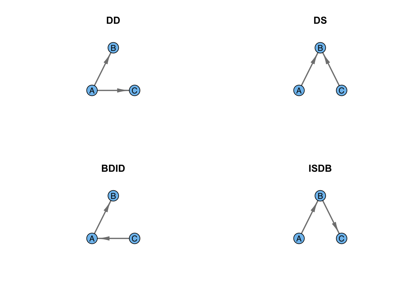
Consequently, transitivity seems to be a sort of default for triadic interactions. This is an interesting observation because it suggests that when there is an excess of 030C triads, some sort of energy has been added to the system. Using data from an experimental hierarchy of chickens, Chase (1982) shows that the majority of triads (17/23) form with the DD sequence, followed by the DS (4/23). The remaining two triads formed by BDID and ISDB (one each).
Chase (1982: 229) suggested that “Winning begets winning”: winners go on to dominate bystanders rather than the other way around. Relationship to testosterone-mediated winner effects?
Since the early work of Simmel, triads have played a central role in structural theories of human action (e.g., Evans-Pritchard (1929) and eventually Heider (1958) on structural balance, Granovetter (1973) on weak ties, Chase (1982) on triads and hierarchies as discussed above, Coleman (1988) on network closure, Burt (1992) on structural holes). However, Faust (2007, 2008, 2010) has shown that >90% of the variance in triad distributions can be accounted for by lower-level features of networks such as edge density and the dyad census. Furthermore, triads have been shown to be highly problematic in regression models for social networks. Inclusion of triangle terms in exponential random graph models makes model degeneracy likely. Handcock (2003) has shown that the constraints on triangles imposed by edge density can be quite severe, making the MCMC-based estimation of ergms very difficult.
Faust (2010) shows that triads are still important. Shared edgewise partnerships save triads in ergms.
In 1929, pioneering British social anthropologist E.E. Evans-Pritchard, known as “EP” to his contemporaries and students, wrote a short paper for Man, the journal of the Royal Anthropological Institute (Evans-Pritchard 1929). He noted a paradox: Sons among the Azande of present-day South Sudan treated their mothers with cool detachment and frequent contempt, despite the fact that Azande mothers would dote on their sons. Why was this? EP’s reasoning is an early example of relational thinking. EP argued that the tense relationship bet: “Therefore to grasp the full meaning of the son-mother relationship we have to take into account not only the whole complex of mutual obligations and privileges standardized modes of behavior, biological and legal affinities and terms of nomenclature composing this relationship, but we have equally to study those which compose the husband-wife and father-son relationships.” The son grows up seeing his father treat his mother with diffidence and contempt and because the favor of the father is all-important for the Zande boy, he aligns his affect with that of his father.
We can represent this triadic relationship using a signed graph, in which the edges of the graph contain weights of \(+1\) if the relationship is positive and \(-1\) if they are negative. Calculating the product of the cycles provides a way of assessing the stability of the structure. If the overall sign of the triad is negative, then its relations are out-of-balance. If they are positive, on the other hand, they are balanced and we expect a more harmonious, stable structure. We can represent the edge weights by coloring the edges green for positive and red for negative. The two stable configurations for a signed triad are either all positive or, as suggested by EP for Zande father-mother-son triads, two negative and one positive.
eplabs <- c("M","S","F")
EP <- graph( c(1,2, 1,3, 2,3), n=3, directed=FALSE)
plot(EP, layout=tri.coords,
     vertex.label=eplabs,
     vertex.label.family="sans",
     vertex.label.color="black",
     vertex.color="white",
     vertex.frame.color="black",
     vertex.size=25,
     edge.width=5,
     edge.color=c("red","red","green"))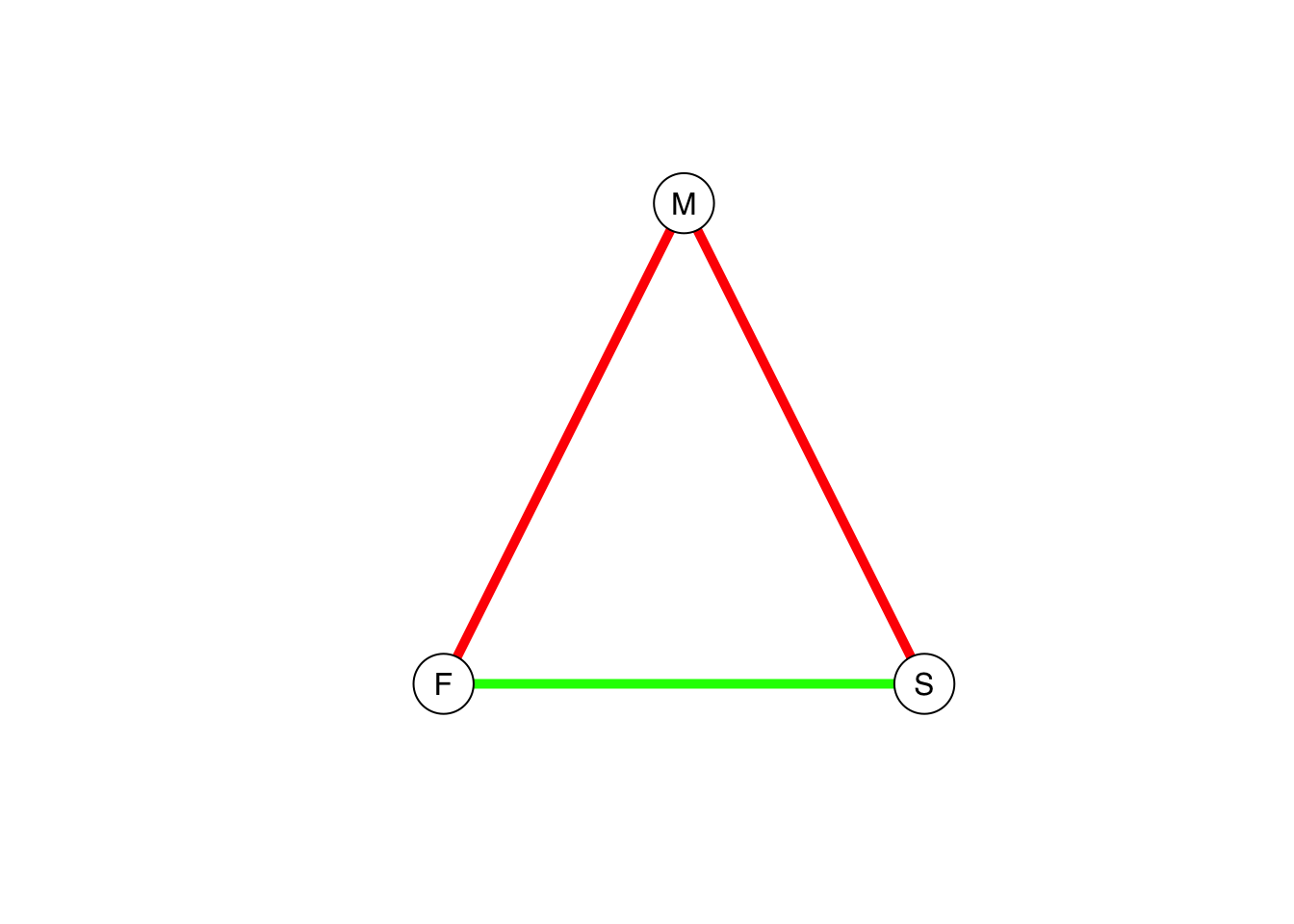
Evans-Pritchard’s idea of the importance of positive cycles was more fully elaborated in Heider’s theory of structural balance. Moody and White biconnectivity, etc.
When we first read a graph into R, it is generally a good idea to explore it a bit to get a sense of its overall properties. The best place to start is with the graph summary. We can use Padgett’s data on Florentine marriages to explore the analysis of graphs using igraph.
flo <- read.table("data/flo.txt",
                  header=TRUE, row.names=1)
gflo <- graph_from_adjacency_matrix(as.matrix(flo), mode="undirected")
gflo
IGRAPH 5364e04 UN-- 16 20 --
+ attr: name (v/c)
+ edges from 5364e04 (vertex names):
[1] Acciaiuoli--Medici Albizzi --Ginori Albizzi --Guadagni
[4] Albizzi --Medici Barbadori --Castellani Barbadori --Medici
[7] Bischeri --Guadagni Bischeri --Peruzzi Bischeri --Strozzi
[10] Castellani--Peruzzi Castellani--Strozzi Guadagni --Lamberteschi
[13] Guadagni --Tornabuoni Medici --Ridolfi Medici --Salviati
[16] Medici --Tornabuoni Pazzi --Salviati Peruzzi --Strozzi
[19] Ridolfi --Strozzi Ridolfi --Tornabuoni plot(gflo, vertex.color="skyblue2",vertex.frame.color="skyblue2",vertex.label.family="Helvetica")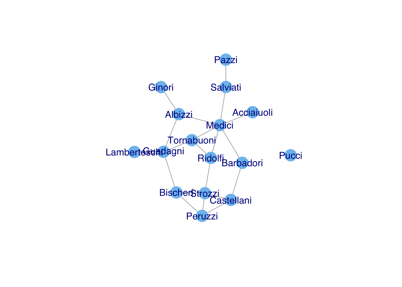
plot(gflo, vertex.shape="none", vertex.label.family="Helvetica")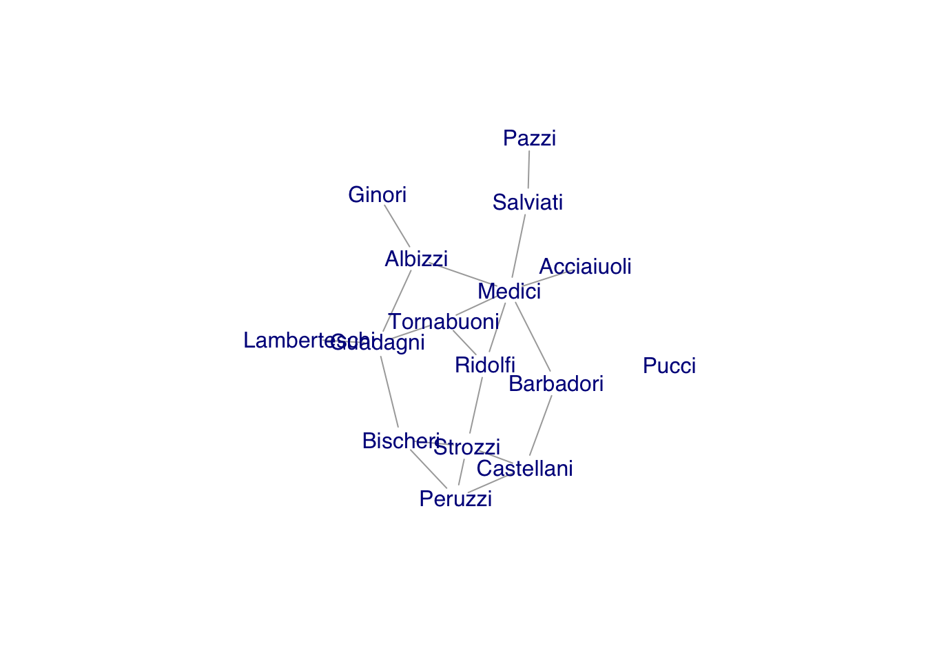
The summary of our graph provides a great deal of information, even if it is a bit terse. The first piece of information is that it is, in fact, an igraph object. Following IGRAPH indicator, we get a one-to-four letter code indicating what type of graph it is. For the Florentine marriage graph, it is of type UN--, which means that it is undirected (U) and named (N). If our graph was weighted, there would be a third letter W and if it were bipartite, the fourth letter would be B. As gflo is neither weighted nor bipartite, the code is only two letters, UN. Following this two-letter code, we get a summary of the number of vertices and edges in the graph, 16 20. There are 16 vertices and 20 edges in gflo. Finally, we see that there is one attribute contained in the graph, + attr: name (v/c). This means that there is a vertex attribute (v) called “name” which is of type character (c).
Given that there are a reasonably small number of vertices and (especially) edges, another good idea to to visualize the graph. In general, it is always a good idea to do this. However, if the graph is really big and has lots of edges, the visualization may take some time so you shouldn’t do it casually. For the Florentine marriages, we have only 16 vertices and 20 edges, so plotting is simple.
One of the first things that we discover when we visualize the Florentine marriage network is that one family, Pucci, is an isolate. There were no marriage ties between the Puccis and any of the other 15 families in Padgett’s sample.
Because the graph is so small, it’s easy to see that Pucci is an isolate. In other cases, it may not be so obvious. There are a number of things we can do to study the overall connectedness of a graph. The first is to ask whether the graph is, in fact, connected. For a graph \(\mathcal{G}\) to be connected, there must be a path between all vertices in \(\mathcal{G}\). If the graph is not connected, we might want to know how many distinct components there are. A component is a maximally connected subgraph of a graph (i.e., a path exists between all vertices in the subgraph). We can find the components of our graph using the igraph function components() (which is a great improvement on its previous instantiation as clusters()!).
is_connected(gflo)[1] FALSEcomponents(gflo)$membership
Acciaiuoli Albizzi Barbadori Bischeri Castellani Ginori
1 1 1 1 1 1
Guadagni Lamberteschi Medici Pazzi Peruzzi Pucci
1 1 1 1 1 2
Ridolfi Salviati Strozzi Tornabuoni
1 1 1 1
$csize
[1] 15 1
$no
[1] 2We can see that gflo is not connected (since we know from visual inspection that Pucci is an isolate). There are two components in gflo: the main component that includes 15 of the 16 families and then a component of one (Pucci), also known as an isolate.
Knowing that the graph is not connected, we can use the command decompose.graph() to extract the elements. In this case, we really only care about the first component, since the second of the two components is simply an isolate.
gflo1 <- decompose(gflo)[[1]]
lay <- layout_with_fr(gflo1)
plot(gflo1, vertex.color="skyblue2", vertex.label=NA, layout=lay)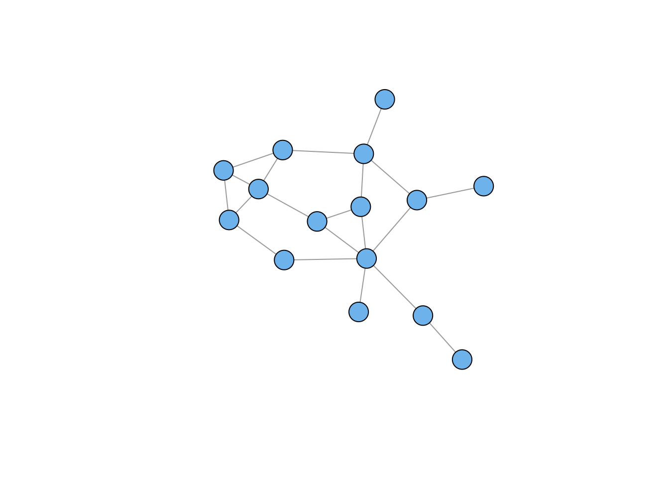
The number of unordered pairs of vertices in a graph of size \(n\) is \(n(n-1)/2\). This means that the density of edges in a graph is simply given by the ratio of the number of observed edges to the number of possible edges, \(2e/n(n-1)\), where \(e\) is the number of edges in the graph.
We can use Padgett’s data on Florentine marriages to explore some of the properties with more complex networks.
Now let’s manually calculate the density of this network:
## note we're working with the matrix, not the graph object here
n <- dim(flo)[1]
2*sum(apply(flo,1,sum)/2)/(n*(n-1))
[1] 0.1666667Here, we summed along the rows of the matrix and then summed the resulting vector to get the number of elements in the sociomatrix. We then divided by two since each marriage is represented twice in the sociomatrix (since it is an undirected relation). Taking out the Pucci isolate, we get a slightly different density. We can use the igraph function graph.density() to reassure ourselves that this is, in fact, the right value. First, however, we will need to remove the unconnected family (Pucci) from the network. We’ll want this later anyway. We can pull out the connected portion of the network using induced_subgraph() starting from any vertex but Pucci.
n <- n-1
2*sum(apply(flo,1,sum)/2)/(n*(n-1))
[1] 0.1904762edge_density(gflo1)[1] 0.1904762In his classic essay, Lin Freeman (1978) lays out the different notions of centrality:
degree centrality captures the idea that individuals with many contacts are central to a structure. This measure is calculated simply as the degree of the individual actor.
closeness centrality captures the idea that a central actor will be close to many other actors in the network. Closeness is measured by the geodesics between actor \(i\) and all others.
betweenness centrality captures the idea that high-centrality individuals should be on the shortest paths between other pairs of actors in a network. The betweenness of actor \(i\) is simply the fraction of all geodesics in the graph on which \(i\) falls.
For non-directed graphs, the degree centrality of vertex \(i\) is simply the sum of edges incident to \(v_i\):
[ C_D(v_i) = d(v_i) = j x{ij} = j x{ji}. ]
Note that while we call this a “centrality” measure, it is simply the degree of node \(i\). Sometimes degree centrality measure will be standardized by the size of the graph \(n\): \(C'_D(v_i) = d(v_i)/(n-1)\), where we subtract one from the size of the graph to account for the actor itself.
For non-directed graphs, the closeness centrality of vertex \(i\) is the inverse of the sum of geodesics between \(v_i\) and \(v_j,~~j\neq i\):
[ C_C(v_i) = ^{-1}, ]
where \(d(v_i, v_j)\) is the distance (measured as the minimum distance or geodesic) between vertices \(i\) and \(j\). Note that if any \(j\) is not reachable from \(i\), \(C_C(v_i)=0\) since the distance between \(i\) and \(j\) is infinite! This means that we often want to restrict our measurements of centrality to connected components of a graph. To standardize, we multiply by \(n-1\), the number of vertices not including \(i\): \(C'_C(v_i) = (n-1) C_C(v_i)\).
For non-directed graphs, the betweenness centrality of vertex \(i\) is the fraction of all geodesics in the graph on which \(i\) lies:
[ C_B(v_i) = g*{jk}(v_i)/g_{jk}, ]
where \(g_{jk}\) is the number of geodesics linking actors \(j\) and \(k\) and \(g_{jk}(v_i)\) is the number of geodesics linking actors \(j\) and \(k\) that contain actor \(i\). It can be standardized by dividing by the number of pairs of actors not including \(i\), \((n-1)(n-2)/2\): \(C'_B(v_i) = C_B(v_i)/[(n-1)(n-2)/2]\).
Another notion of centrality is that a central person is someone who knows people who know a lot of people. This idea can be captured using a measure known as information centrality. The calculation of information centrality is a bit more complicated than for the other three measures and requires some linear algebra. Start with the sociomatrix \(\mathbf{X}\). From this, we calculate an intermediate matrix \(\mathbf{A}\). For a binary relation, \(a_{ij}=0\) if \(x_{ij}=1\) and \(a_{ij}=1\) if \(x_{ij}=0\) for \(i \neq j\) (that is, the non-diagonal elements of \(\mathbf{A}\) are the complements of their values in \(\mathbf{X}\)). The diagonal elements of \(\mathbf{A}\) (\(a_{ii}\)) are simply the degree of vertex \(i\) plus one, \(a_{ii} = d(v_i)+1\). Once we have \(\mathbf{A}\), we invert it yielding a new matrix \(\mathbf{C}\mathbf{A}^{-1}\). We then calculate \(T\), the trace of \(\mathbf{C}\), which is simply the sum of its diagonal elements and \(R\) which is one of the row sums of \(\mathbf{C}\) (they are all the same). Information centrality is then simply
[ C_I(v_i) = , ]
where, as usual, \(d(v_i)\) is the degree of vertex \(i\) and \(n\) is the size of the graph.
There is no implementation of information centrality in igraph. This can be calculated either in sna or using the following function, which takes a sociomatrix as its only argument. It assumes that the matrix is binary.
infocentral <- function(X){
  ## assumes binary relation
  k <- dim(X)[1]
  A <- matrix(as.numeric(!X),nr=k,nc=k)
  diag(A) <- apply(X,1,sum)+1
  C <- solve(A)
  T <- sum(diag(C))
  R <- apply(C,1,sum)[1]
  ic <- 1/(diag(C) + (T - 2*R)/k)
  return(ic)
}Yet another approach to centrality was suggested by Bonacich (1972). He suggests that the eigenvectors of the sociomatrix are a fruitful way of thinking about centrality. As with information centrality, the eigenvector approach captures the idea that central people will have well-connected alters but that the relative importance of these alters falls off with distance from ego. While the eigenvector (preferably the dominant one) of the sociomatrix is an excellent measure of centrality, the metric Bonacich (1987) suggests is actually a bit more complex:
[ C(,) = ( - )^{-1} , ]
where \(\alpha\) is a parameter, \(\beta\) measures the extent to which an actor’s status is a function of the statuses of its alters decay of influence from the focal actor, \(\mathbf{I}\) is an identity matrix of the same rank as the sociomatrix \(\mathbf{X}\), and \(\mathbf{1}\) is a column vector of ones.
The size of \(\beta\) determines the degree to which Bonacich centrality is a measure of local or global centrality. When \(\beta=0\), only an actor’s direct ties are taken into account – Bonacich centrality becomes proportional to degree centrality. However, when \(\beta>0\), an actor’s alters’ ties are also taken into account. The larger the value of \(\beta\), the more distant ties will matter. It is also possible for \(\beta\) to be less than zero. In this case, being connected to powerful alters who themselves have many alters negatively affects an actor’s status. This seemingly odd situation captures the effect observed in bargaining experiments performed on networks by Cook et al. (1983), where an individual’s ability to negotiate a favorable outcome is lessened when he or she must bargain with powerful, well-connected alters.
Consider the centrality measures on Padgett’s Florentine marriage data. For these analyses, we will take out the Pucci family since they are an isolate. For the standard centrality measures discussed by Freeman, Pucci will have a score of zero. Information and eigenvalue centrality only work on connected graphs.
## infocentral needs matrix, so trim off Pucci from flo
flo1 <- flo[-12,-12]
ic <- infocentral(flo1)
CE <- abs(power_centrality(gflo1))

measures <- cbind(CD=degree(gflo1),
              CB=round(betweenness(gflo1),1),
              CC=round(closeness(gflo1),2),
              CI=round(ic,2),
              CE=round(CE,2))
dimnames(measures)[[1]] <- dimnames(flo1)[[1]]
measures
CD CB CC CI CE
Acciaiuoli 1 0.0 0.03 0.55 0.37
Albizzi 3 19.3 0.03 0.83 2.02
Barbadori 2 8.5 0.03 0.76 1.47
Bischeri 3 9.5 0.03 0.83 0.00
Castellani 3 5.0 0.03 0.79 1.29
Ginori 1 0.0 0.02 0.48 1.84
Guadagni 4 23.2 0.03 0.92 0.18
Lamberteschi 1 0.0 0.02 0.51 0.00
Medici 6 47.5 0.04 1.06 0.55
Pazzi 1 0.0 0.02 0.39 0.00
Peruzzi 3 2.0 0.03 0.78 0.55
Ridolfi 3 10.3 0.04 0.90 1.29
Salviati 2 13.0 0.03 0.60 0.18
Strozzi 4 9.3 0.03 0.88 0.18
Tornabuoni 3 8.3 0.03 0.90 1.10# Plot the graph one last time with the vertices sized according to
# betweenness centrality
plot(gflo1, vertex.size=measures[,"CB"]+1, vertex.color="plum", vertex.label=NA, layout=lay)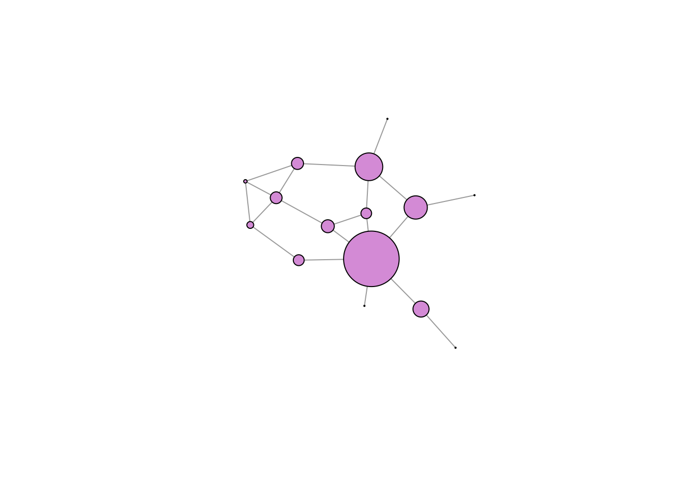
While centrality measures capture different notions of centrality, power, prestige, etc., they are generally fairly highly correlated. This said, some measures can be quite divergent. We can see this with eigenvalue centralities of the Florentine families. The Medici are clearly central to this marriage network. However, because they are so dominant, their alters do not have as many connections as they do. As a result, the Medici have a low eigenvalue centrality, but the Albizzi do quite well.
## correlation matrix of the centralities
cor(measures)
CD CB CC CI CE
CD 1.00000000 0.84392220 0.7463380 0.9207909 -0.02813901
CB 0.84392220 1.00000000 0.6592939 0.7143692 0.01003666
CC 0.74633802 0.65929385 1.0000000 0.8238569 0.12584573
CI 0.92079092 0.71436925 0.8238569 1.0000000 0.14762599
CE -0.02813901 0.01003666 0.1258457 0.1476260 1.00000000## vertex size proportional to eigenvalue centrality
plot(gflo1, vertex.size=measures[,"CE"]*10, vertex.color="plum", vertex.label=NA, layout=lay)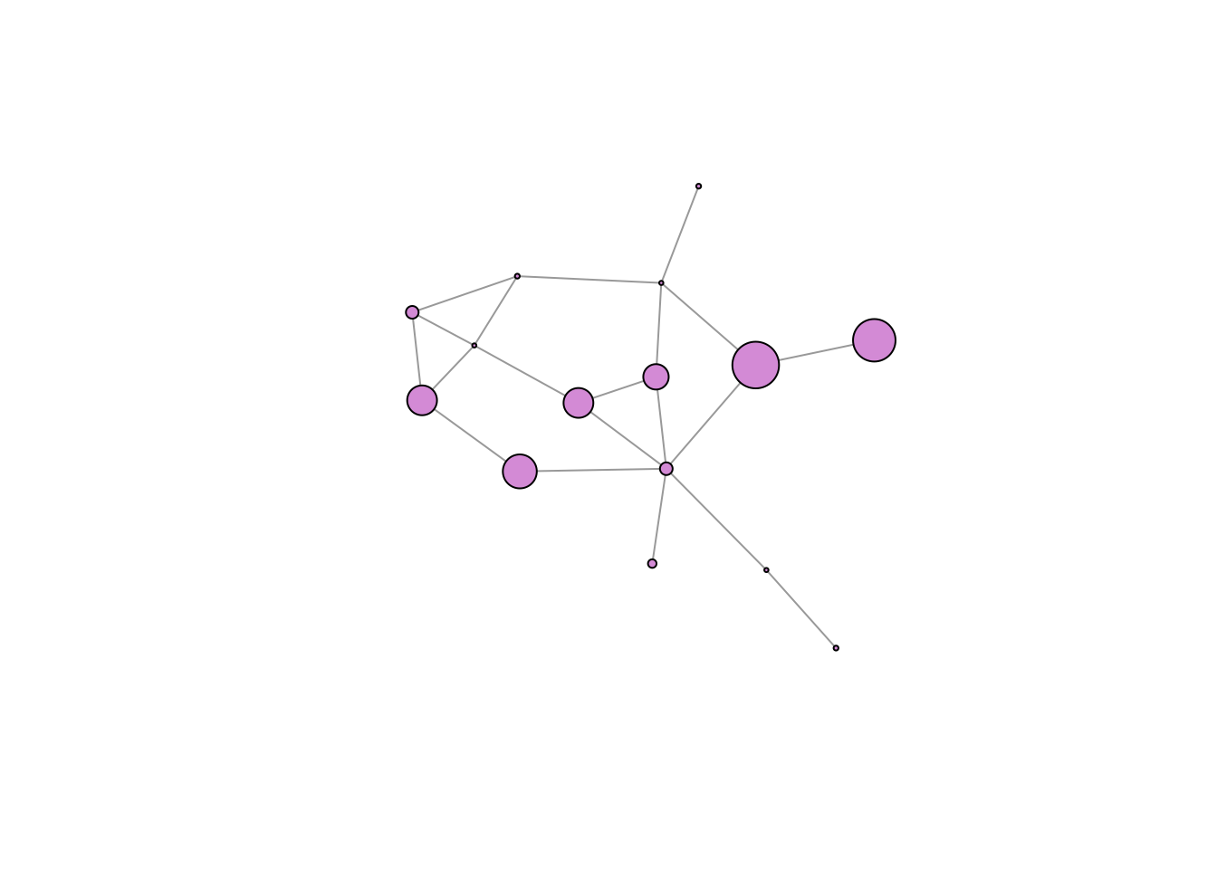
Centralities can be on very different scales and, for some measures, the values can be so wildly different, that they are impractical for scaling vertex size for plotting. For example, betweenness centrality varies between zero and 47.5. We can write a simple function to rescale a variable to make it more useful for plotting.
rescale <- function(x,a,b,c,d) c + (x-a)/(b-a)*(d-c)
bb <- rescale(measures[,2], 0, 47.5, 1, 40)
plot(gflo1, vertex.size=bb, vertex.color="plum", vertex.label=NA, layout=lay)
When plotting graphs, we frequently want to identify some induced subgraph. This might be an ego network or a path such as a link-tracing sample or geodesic.
This can be tricky, particularly if the graph is large. Here are a couple of hacks that help.
We can illustrate how to do this using an example discussed in a forthcoming paper by Turner et al. (2023). In this paper, we show look at the spread and persistence of adaptations in populations characterize by minority-majority-structure and moderate degrees of in-group preference (i.e., homophily). We show that innovations are more likely to spread and be maintained when they arise in minority sub-populations than when they arise in the majority subpopulation. Furthermore, we show that minority-majority structure with moderate homophily is more effective at promoting adaptation than are populations with more equal-sized groups and weak homophily. To try to understand why this might be the case, we can highlight the ego networks of individuals in the minority and majority populations.
We’ll start by constructing a simple minority-majority network and plot that. To do this, we will construct two random graphs – one large, one small – using the function sample_gnm(), which constructs a random graph of \(n\) vertices with \(m\) edges. We then combine them using the discrete-union function %du% and get rid of any isolates (which are common when you construct random graphs). For these sorts of visualizations, it’s very important to have a fixed graph layout, so you can see
set.seed(8675309)
g1 <- sample_gnm(20,60)
g2 <- sample_gnm(200,500)
gg <- g1 %du% g2

## add links across communities
s1 <- sample(1:20,5,replace=FALSE)
s2 <- sample(21:220,5,replace=FALSE)
gg <- add_edges(gg,c(rbind(s1,s2)))

## only the connected component
gg <- induced_subgraph(gg, subcomponent(gg,1))

## plotting
cols <- c(rep("blue4",20), rep("magenta",200))
ecols <- rep("#A6A6A6",565)
lay <- layout_with_fr(gg)


plot(gg, vertex.size=5,
    vertex.color=cols,
    vertex.frame.color=cols,
    vertex.label=NA,
    edge.width=0.5,
    edge.color=ecols,
    layout=lay)
Next, we’ll highlight an individual in the minority population who has a tie to the majority population.
We want to highlight an ego network embedded within a larger graph. We can use the function make_ego_graph() to extract the ego network but it will renumber all the vertices and edges, making it useless for subsetting the larger graph for visualization. The key piece of information is that functions like make_ego_graph() and induced_subgraph() retain all the vertex/edge covariate values of the original graph. We can therefore construct vertex and edge counters and assign these as attributes.
This is probably considered a feature, but it can feel more like a bug if you’re not expecting it. make_ego_graph() returns a list regardless of how many vertices you give it in the nodes argument. You need to extract the graph object using double square brackets, as usual for extracting list elements.
We pick a vertex 10 (having already ascertained which vertices have ties across groups) and calculate its second-order ego network (i.e., all of 10’s connections plus all their connections). We will color ego (i.e., node 10) cyan, ego’s second-order ego network blue. Everything else remains the same.
# highlight ego network in minority group
E(gg)$id <- seq_len(ecount(gg))
V(gg)$vid <- seq_len(vcount(gg))
ego10 <- make_ego_graph(gg,order=2,nodes=10)
ego10 <- ego10[[1]]
##
cols1 <- cols
cols1[V(ego10)$vid] <- "blue"
cols1[10] <- "cyan"
ecols1 <- ecols
ecols1[E(ego10)$id] <- "blue"

## plotting
plot(gg, vertex.size=5,
   vertex.color=cols1,
   vertex.frame.color=cols1,
   vertex.label=NA,
   edge.width=0.5,
   edge.color=ecols1,
layout=lay) 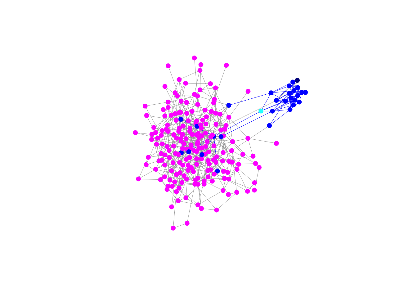
Vertex 10 has several connections to individuals in the majority population. Moreover, they are connected to nearly everyone in the minority population.
Now we can look at a corresponding ego network in the majority group. We will focus on vertex 153, which is in the core of the majority network.
# highlight corresponding ego network in majority group
ego153 <- make_ego_graph(gg,order=2,nodes=153)
ego153 <- ego153[[1]]

cols2 <- cols
cols2[V(ego153)$vid] <- "blue"
cols2[153] <- "cyan"
ecols2 <- ecols
ecols2[E(ego153)$id] <- "blue"

plot(gg, vertex.size=5,
     vertex.color=cols2,
     vertex.frame.color=cols2,
     vertex.label=NA,
     edge.width=0.5,
     edge.color=ecols2,
layout=lay) 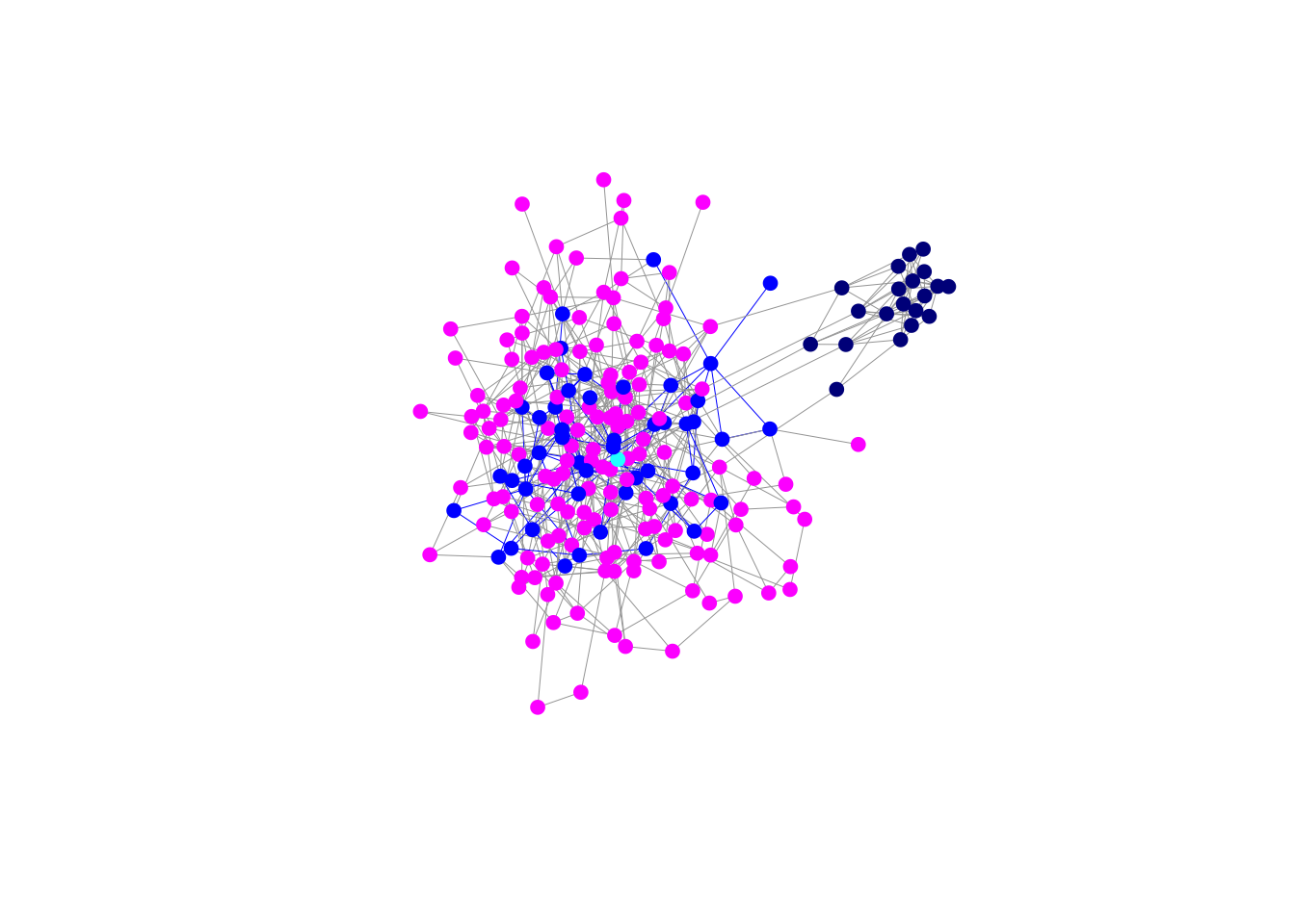
Because vertex 153 is in the core of the majority network, its second-order ego network is quite extensive. However, note that it does not have any ties whatsoever to the minority group.
People tend to be skeptical of innovation. You are unlikely to adopt a major change to your livelihood (as an adaptation to climate change may very well be) from just anyone. Presumably, if you are going to adopt an innovation, it will need to come from a trusted, authoritative source. As suggested by Centola (2019), you need to have wide bridges for innovation to spread, but deviance (even if positive) tends to be suppressed in the dense, cohesive cores of societies (Coleman 1988). This makes strongly-connected, cohesive groups unlikely sources of innovation, even though the cohesiveness suggests that trust should be high. Is there any part of this network away from the core where there are nonetheless wide bridges? Yes. It’s on the periphery, in the liminal space between the minority and majority communities. Members of the majority community with any ties to the minority community are likely to see multiple models of some innovation from their contacts with the minority population.
Note that 25% of the minority group have ties to the majority group, whereas only 2.5% of the vertices of the majority group have any ties to the minority group. 8% of the total number of edges incident to the minority group are cross-group ties. Compare that to 1% cross-group ties for the majority population.