#library(devtools)
# install_github("zalmquist/networkdata")
library(networkdata)5 Exponential Random Graph Models
5.1 What is an ERGM?
ERGM stands for Exponential Random Graph Model
The goal of ERGMs is to “describe parsimoniously the local selection forces that shape the global structure of a network” (Hunter et al. 2008)
ERGMs are analogous to logistic regression: they predict the probability that a pair of nodes in a network will have a tie between them, but they have some important differences from standard regression methods
ERGMs can be used for directed, undirected, valued, unvalued, and bipartite networks.
5.2 Why not use standard regression methods?
5.2.1 Some practical reasons
- ERGMs can be used to simulate similar networks as well as to conduct regression-like analyses
- ERGMs more intuitively allow you to include interactions between individual attributes at the dyadic level, as well as edge attributes and predictor networks
5.2.2 Theoretical reasons
- Ties between nodes in real social networks are not independent; for example, as we’ve seen, reciprocity and transitivity are common features of human social networks.
- This non-independence violates the most basic assumption of regression!
- Through simulation, ERGMs allow dyadic and higher-order dependencies to be modeled.
- Treating individuals as independent of their social context is a very strange thing to do from an anthropological perspective.
5.3 What is a random graph?
Imagine a network with (n) nodes.
Edges between nodes could occur randomly with probability (p) (each potential edge is one Bernoulli trial).
Network density, or the number of edges in observed network divided by the number of possible edges, is usually used for (p).
In this case, the degree of any node is binomially distributed (with (n-1) Bernoulli trials per node, for a directed graph).
This type of homogeneous Bernoulli graph is often referred to as an “Erdős-Rényi” graph. These random graphs are the “null” hypothesis of an ERGM.
5.4 ERGMs
Let () denote an (n n) sociomatrix where (y_{ij}=1) if individuals (i) and (j) have a tie.
Let () denote a matrix of covariates, which includes structural measures of the network as well as nodal and possibly edge-level attributes.
A generic ERGM can be written as:
\[ P_{\theta, \mathcal{Y}}(\mathbf{Y = y| X}) = \frac{\exp\{ \theta^{\textsf{T}} g(y, X)\}}{\kappa(\theta, \mathcal{Y})},\]
where \(\theta\) is a vector of coefficients,
\(g(y, \mathbf{X})\) is a vector of sufficient statistics,
\(\mathcal{Y}\) is the space of possible graphs,
\(\kappa(\theta, \mathcal{Y})\) is a normalizing constant (i.e., it’s the numerator summed across all possible graphs \(\mathcal{Y}\))
For even moderate \(n\), \(\kappa(\theta, \mathcal{Y})\) can be enormous, so closed-form solutions are unfeasible.
The number of labeled, undirected graphs of \(n\) vertices is \(2^{n(n-1)/2}\), which can get big fast.
For example, for a network of \(n>7\), there are over two million undirected graphs (\(2^{21}\)), which means that you would need to calculate the likelihood for each one of these in order to compute \(\kappa\).
This is generally not practical for even moderately-sized graphs.
5.5 Some Definitions and Notation
\(y_{ij}\) denotes the \(ij\)th dyad in graph \(y\) if \(y_{ij}=1\), then \(i\) and \(j\) are connected by an edge, if \(y_{ij}=0\), they are not.
\(y^c_{ij}\) is the status of all other pairs of vertices in \(y\) other than \((i,j)\).
\(y^+_{ij}\) is the same network as \(y\) except that \(y_{ij}=1\).
\(y^-_{ij}\) is the same network as \(y\) except that \(y_{ij}=0\).
\(\delta(y_{ij})\) is the change statistic: \(\delta(y_{ij})=g(y^+_{ij}) - g(y^-_{ij})\). This is a measure of how the graph statistic \(g(y)\) changes if the \(ij\)th vertex is toggled on or off.
The ergm equation can be re-written in terms of change statistics.
The log-odds of a tie \(y_{ij}\) is:
\[ \operatorname{logit}(Y_{ij}=1\|y^c_{ij}) = \theta^{\textsf{T}} \delta(y_{ij}) \]
- (why is the \(Y\) capitalized? because we are looking at the random variable \(Y_{ij}\) rather than the specific realization)
5.6 Getting Started
Zack Almquist has put together Lin Freeman’s collection of network data in his
networkdatapackage, which is on github and can be installed usingRdevtools.I commented out the
library(devtools)andinstall_github()command in these notes because I already have the package installed!
5.7 Bott Nursery School Data
- We will use the data from a paper by H. Bott in 1928 that used ethological observations of children in a nursery school (Bott 1928). The Bott data actually contain five sets of relations:
- talked to another child
- interfered with another child
- watched another child
- imitated another child
- cooperated with another child
- These are organized into a “graph stack,” which is essentially a specialized
listfor storing network data used by thenetworkpackage.
library(statnet)
data(bott)
summary(bott)
Length Class Mode
talk 5 network list
interfere 5 network list
watch 5 network list
imitate 5 network list
cooperate 5 network listbott$talk
Network attributes:
vertices = 11
directed = TRUE
hyper = FALSE
loops = FALSE
multiple = FALSE
bipartite = FALSE
total edges= 75
missing edges= 0
non-missing edges= 75
Vertex attribute names:
age.month vertex.names
Edge attribute names:
edgevalue
$interfere
Network attributes:
vertices = 11
directed = TRUE
hyper = FALSE
loops = FALSE
multiple = FALSE
bipartite = FALSE
total edges= 72
missing edges= 0
non-missing edges= 72
Vertex attribute names:
age.month vertex.names
Edge attribute names:
edgevalue
$watch
Network attributes:
vertices = 11
directed = TRUE
hyper = FALSE
loops = FALSE
multiple = FALSE
bipartite = FALSE
total edges= 51
missing edges= 0
non-missing edges= 51
Vertex attribute names:
age.month vertex.names
Edge attribute names:
edgevalue
$imitate
Network attributes:
vertices = 11
directed = TRUE
hyper = FALSE
loops = FALSE
multiple = FALSE
bipartite = FALSE
total edges= 35
missing edges= 0
non-missing edges= 35
Vertex attribute names:
age.month vertex.names
Edge attribute names:
edgevalue
$cooperate
Network attributes:
vertices = 11
directed = TRUE
hyper = FALSE
loops = FALSE
multiple = FALSE
bipartite = FALSE
total edges= 23
missing edges= 0
non-missing edges= 23
Vertex attribute names:
age.month vertex.names
Edge attribute names:
edgevalue plot(bott[[1]]) # talked to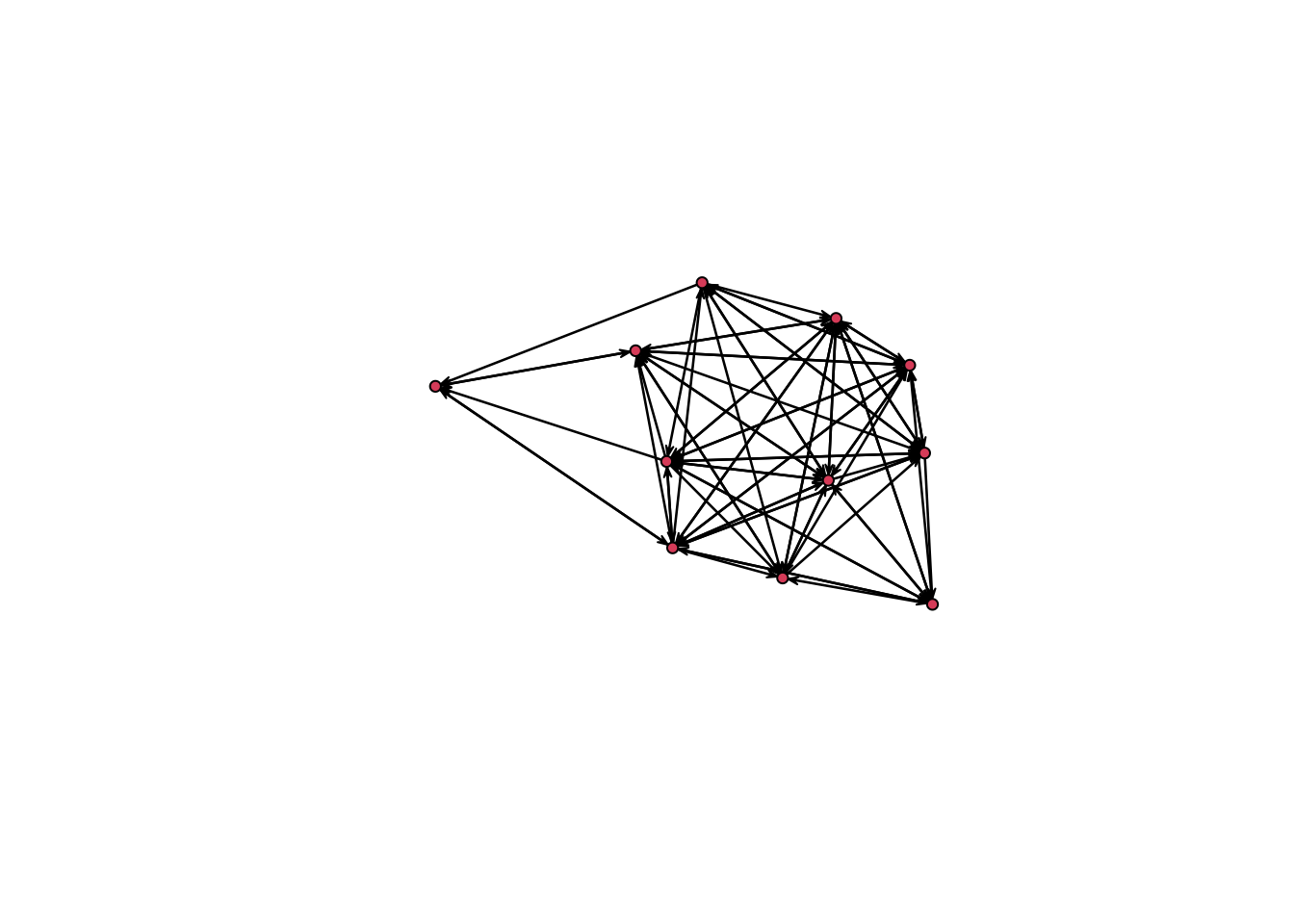
plot(bott[[2]]) # interfered with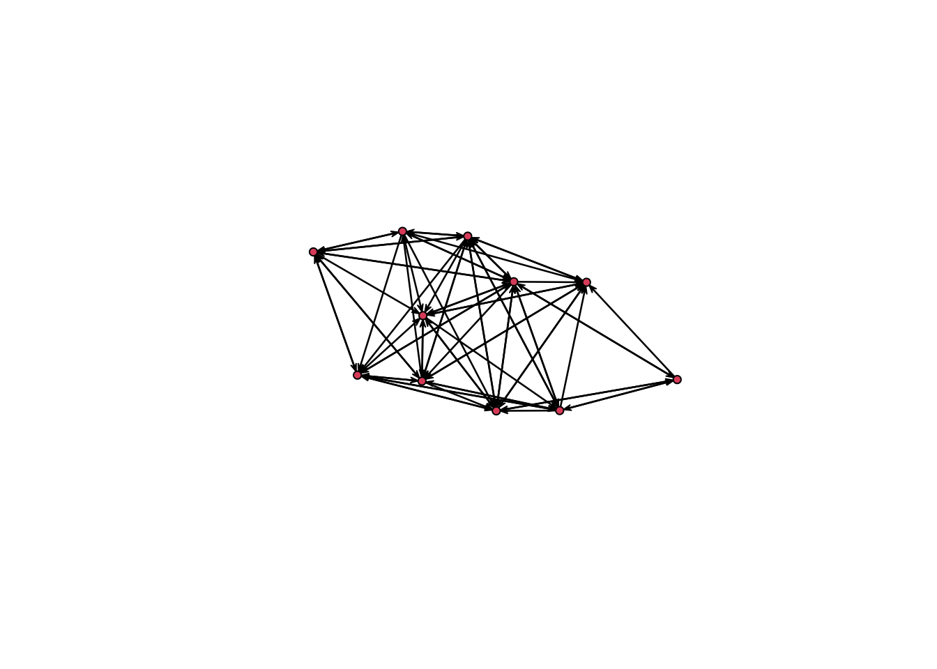
plot(bott[[3]]) # watched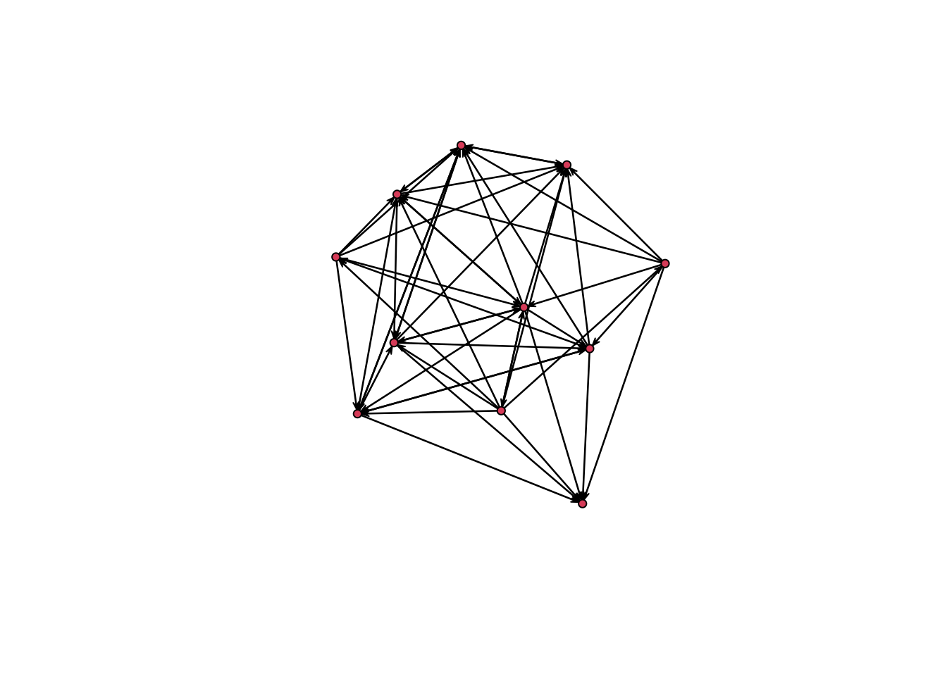
plot(bott[[4]]) # imitated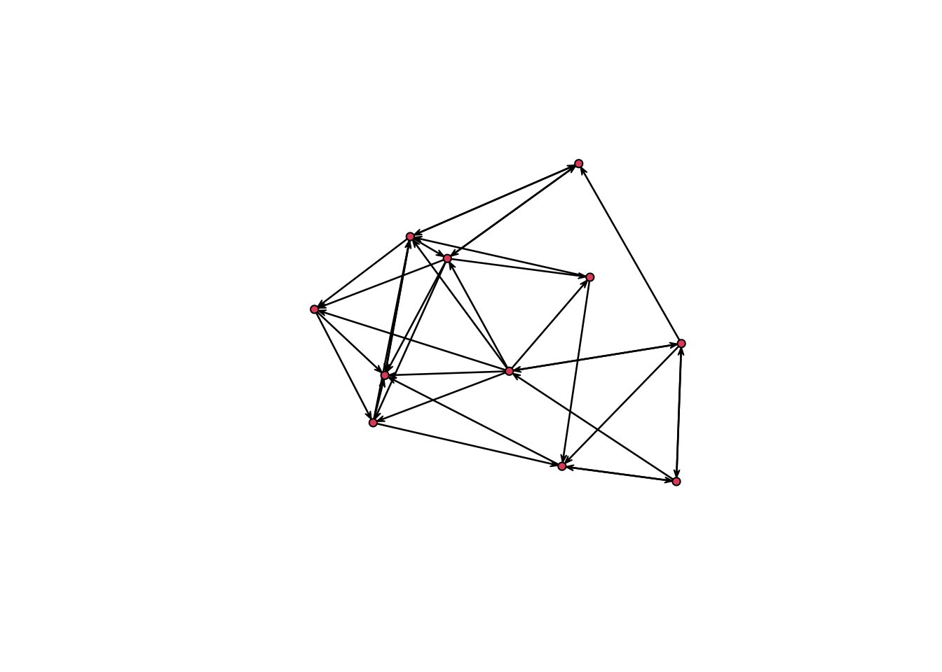
plot(bott[[5]]) # cooperated with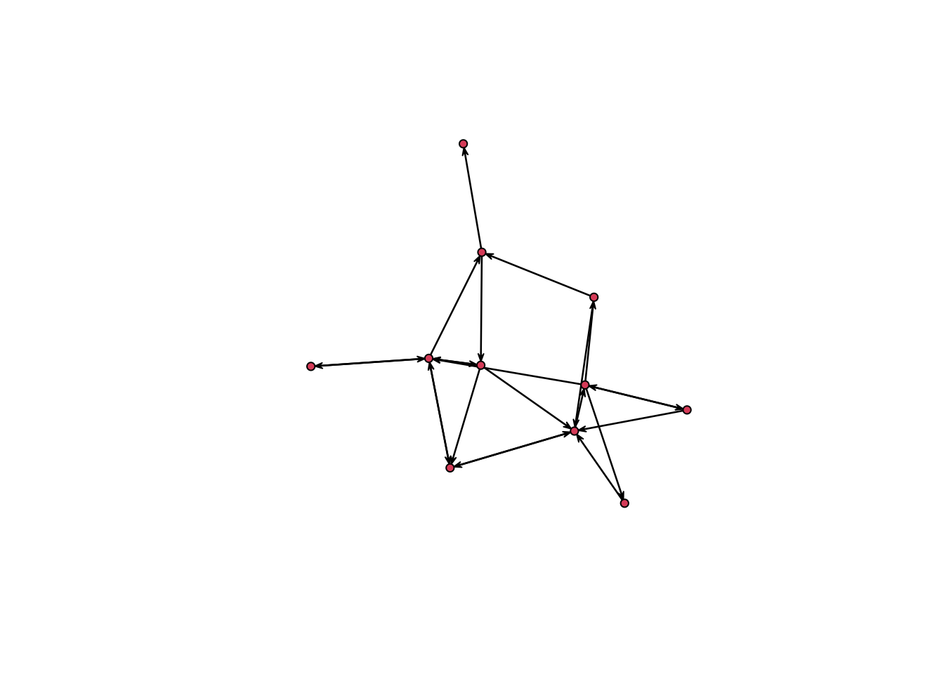
We can see that the first three relations yield quite dense networks (note that ergms would not tell us much in this case!).
We will work first with the imitation network.
The first thing we’ll do is fit a model that just has edges in it. This is kind of like fitting a regression model with only an intercept.
summary(bott[[4]]~edges) # how many edges?edges
35 bottmodel.01 <- ergm(bott[[4]]~edges) # Estimate minimal modelStarting maximum pseudolikelihood estimation (MPLE):Obtaining the responsible dyads.Evaluating the predictor and response matrix.Maximizing the pseudolikelihood.Finished MPLE.Evaluating log-likelihood at the estimate. summary(bottmodel.01) # The fitted model objectCall:
ergm(formula = bott[[4]] ~ edges)
Maximum Likelihood Results:
Estimate Std. Error MCMC % z value Pr(>|z|)
edges -0.7621 0.2047 0 -3.723 0.000197 ***
---
Signif. codes: 0 '***' 0.001 '**' 0.01 '*' 0.05 '.' 0.1 ' ' 1
Null Deviance: 152.5 on 110 degrees of freedom
Residual Deviance: 137.6 on 109 degrees of freedom
AIC: 139.6 BIC: 142.3 (Smaller is better. MC Std. Err. = 0)5.8 The Allure of Triangles
Triads are really important for understanding social relations. Some important roles for triads:
- hierarchy
- network closure
- brokerage
- exclusion
- generalized exchange
- bystander effects
- forbidden relationships
- filial loyalties
Starting with the work of Davis, Holland, Leinhardt, we know that one of the principle differences between empirical social networks and random graphs is the pattern of triads in human social networks.
Put simply, there are far more triangles, and particularly transitive triads, in social networks than would be expected from random graphs of similar density.
5.9 Transitive Triads
Empirically, we know a number of things about transitive triads in particular:
- friendships tend to be overwhelmingly transitive (Holland and Leinhardt 1971)
- children show increasing tendencies for transitivity as they get older (Leinhardt 1972)
- higher agreement between pairs within transitive triads (Krackhardt and Kilduff 2002)
- adolescents in intransitive friendship triads have more suicidal ideations (Bearman and Moody 2004)
Furthermore, the presence of intransitive triads is itself important. Yeon Jung Yu (2016) showed that sex workers on Hainan Island, China, who overwhelmingly tend to be migrants from rural areas, have a large number of intransitive friendship triangles.
These are the 201 triangles that, e.g., Davis (1970) and Davis and Leinhardt (1972) find missing in most human networks.
Yu interpreted as arising because of the need to manage information about these women’s activities away from home – “forbidden” triangles are common because of active management.
Triangles measure transitivity and clustering in networks.
We can add a triangle term to our ergm.
Unlike the edges-only model, this model will need to be estimated via MCMC.
summary(bott[[4]]~edges+triangle) edges triangle
35 40 bottmodel.02 <- ergm(bott[[4]]~edges + triangle)Starting maximum pseudolikelihood estimation (MPLE):Obtaining the responsible dyads.Evaluating the predictor and response matrix.Maximizing the pseudolikelihood.Finished MPLE.Starting Monte Carlo maximum likelihood estimation (MCMLE):Iteration 1 of at most 60:Warning: 'glpk' selected as the solver, but package 'Rglpk' is not available;
falling back to 'lpSolveAPI'. This should be fine unless the sample size and/or
the number of parameters is very big.1Optimizing with step length 1.0000.The log-likelihood improved by 0.0489.Convergence test p-value: 0.0002. Converged with 99% confidence.
Finished MCMLE.
Evaluating log-likelihood at the estimate. Fitting the dyad-independent submodel...
Bridging between the dyad-independent submodel and the full model...
Setting up bridge sampling...
Using 16 bridges: 1 2 3 4 5 6 7 8 9 10 11 12 13 14 15 16 .
Bridging finished.
This model was fit using MCMC. To examine model diagnostics and check
for degeneracy, use the mcmc.diagnostics() function.summary(bottmodel.02)Call:
ergm(formula = bott[[4]] ~ edges + triangle)
Monte Carlo Maximum Likelihood Results:
Estimate Std. Error MCMC % z value Pr(>|z|)
edges -0.56345 0.54626 0 -1.031 0.302
triangle -0.05671 0.14551 0 -0.390 0.697
Null Deviance: 152.5 on 110 degrees of freedom
Residual Deviance: 137.5 on 108 degrees of freedom
AIC: 141.5 BIC: 146.9 (Smaller is better. MC Std. Err. = 0.01803)You will notice that as we move from the edges-only model to the edges-plus-triangles, the estimation method changes.
Edges are dyad-independent so we can estimate the model simply using MPLE.
This is basically fitting a logistic regression to our network ties.
In contrast, triangles are a dyad-dependent term and the ergm must be fit using MCMC simulation.
Depending on the size of your network, this might take a while.
5.10 Degeneracy
Whenever
ergmfits a model via MCMC, you will get a warning telling you to check for degeneracy and model diagnostics.If the model shows clear signs of degeneracy, you will receive a warning.
- but don’t assume that if you don’t get a warning that the model is fine – always check the goodness-of-fit.
In general, triangles cause problems in ergms.
They often lead to a phenomenon known as degeneracy.
While our intuition tells us that triangles should matter for networks – because triangles result from transitivity – it turns out that there are better ways to represent transitivity in network models.
A series of papers by Katie Faust (2007, 2008, 2010) shows that triadic structures are highly constrained by lower-level structures, namely, edge density.
In the limited-choice paradigm employed by Ad Health (i.e., “name your five best female/male friends”), Faust (2010) found that the triad census in 128 networks was almost perfectly explained by one dimension of a multivariate analysis (conceptually similar to the loading on a principal component) and that edge density accounted for 96% of the variance in locations along this dimension!
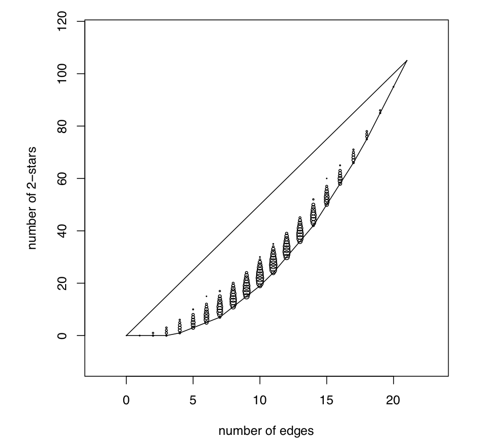
This result was extreme – and determined in large part by the analysis of restricted-choice questions for a single relation – but the point remains: the number (and pattern) of triads in a network will be highly constrained by the number of edges and the size of the network, which jointly determine the network density.
In a very important working paper, Mark Handcock showed that this situation of extreme constraint causes the MCMC algorithm by which ergms are estimated to behave badly, leading to the condition of degeneracy discussed above.
A network model is degenerate when the space that an MCMC sampler can explore the network space is so constrained that the only way to get the observed \(g(y)\) is essentially to flicker between full and empty graphs in the right proportion.
Handcock (2003) showed this in what came to be known as his “stealth bomber” plot of the probability of degeneracy for an edges-and-triangles ERGM
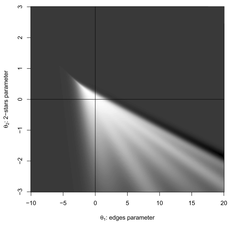
Not what you want out of an MCMC estimator.
A good indication that you have a degenerate model is that you have
NAvalues for standard errors on your ergm parameter estimates. You can’t calculate a variance – and, therefore, a standard error – if you simply flicker between full and empty graphs.The upshot of this is that, despite our strong intuitions about the importance of triadic interactions in determining social structure, I do not recommend using the
triangleterm in ergms. There are better alternatives, which we will discuss later.
5.11 Nodal Covariates
We often have a situation where we think that the attributes of the individuals who make up our graph vertices may affect their propensity to form (or receive) ties.
To test this hypothesis, we can employ nodal covariates using the
nodecov()term.
age <- bott[[4]] %v% "age.month"
summary(age) Min. 1st Qu. Median Mean 3rd Qu. Max.
26.00 33.50 38.00 40.09 48.50 54.00 plot(bott[[4]], vertex.cex=age/24)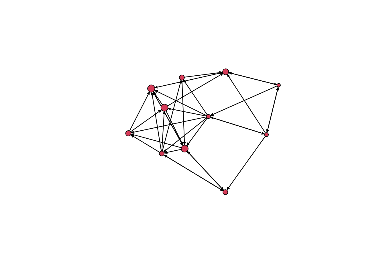
summary(bott[[4]]~edges+nodecov('age.month')) edges nodecov.age.month
35 2842 bottmodel.03 <- ergm(bott[[4]]~edges+nodecov('age.month'))Starting maximum pseudolikelihood estimation (MPLE):Obtaining the responsible dyads.Evaluating the predictor and response matrix.Maximizing the pseudolikelihood.Finished MPLE.Evaluating log-likelihood at the estimate. summary(bottmodel.03)Call:
ergm(formula = bott[[4]] ~ edges + nodecov("age.month"))
Maximum Likelihood Results:
Estimate Std. Error MCMC % z value Pr(>|z|)
edges -1.526483 1.335799 0 -1.143 0.253
nodecov.age.month 0.009501 0.016352 0 0.581 0.561
Null Deviance: 152.5 on 110 degrees of freedom
Residual Deviance: 137.3 on 108 degrees of freedom
AIC: 141.3 BIC: 146.7 (Smaller is better. MC Std. Err. = 0)An extremely important class of nodal covariates are the homophily terms.
Homophily refers to the tendency for people to sort on socio-demographic attributes.
In evolutionary biology, we are probably more familiar with the term assortative mating, which refers to the tendency for mating pairs to form deferentially based on some observable feature of their phenotype.
Indeed, the classic demographic studies of homophily focus on marriage.
Humans show a tendency to assort on all manner of attributes: age, educational status, race, ethnicity, religion, etc.
Attribute-based mixing is extremely important for diffusion processes on networks (e.g., infectious disease or cultural transmission).
Strong homophily in a network can slow down overall diffusion compared to a well-mixed model and can create pockets of high prevalence.
There are two broad flavors of homophily: uniform and differential.
Consider the case of assortative mating based on ethnicity.
Uniform homophily refers to the tendency for people to form sexual unions with people of the same ethnicity and is the same regardless of which ethnicity is considered.
Differential homophily accounts for the fact that the assortative tendencies of sexual partnerships are different depending on the ethnicities of the individuals involved.
In the United States, homophilous (or “ethnically-concordant”) partnerships are much more likely among African Americans than among white couples.
We can look at some data from the 1992 NHSLS on women’s sex partners
library(knitr)
white <- c(1131,12,16,3,15)
black <- c(5,268,5,0,0)
hispanic <- c(39,1,115,0,3)
asian <- c(12,0,0,10,4)
other <- c(7,0,1,0,18)
sp <- rbind(white,black,hispanic,asian,other)
dimnames(sp)[[2]] <- c("white","black","hispanic","asian","other")
kable(sp)| white | black | hispanic | asian | other | |
|---|---|---|---|---|---|
| white | 1131 | 12 | 16 | 3 | 15 |
| black | 5 | 268 | 5 | 0 | 0 |
| hispanic | 39 | 1 | 115 | 0 | 3 |
| asian | 12 | 0 | 0 | 10 | 4 |
| other | 7 | 0 | 1 | 0 | 18 |
We can see that the great majority of partnerships involve white women and men.
The tendency for ethnically concordant-partnerships is also evident as the largest values in any given row/column always lie along the diagonal.
For this sample, it appears that hispanic women and hispanic men are the most “versatile”, having the largest fraction of ethnically-discordant partnerships (though the majority of Asian women’s partnerhsips are actually discordant, which could be another measure of versatility).
We can talk about this some more later, now back to ERGMs…
Unfortunately, the Bott data set does not have any nodal covariates that lend themselves to either
nodematch()ornodemix().
5.12 Reciprocity
Reciprocity is a common relation that we wish to investigate in anthropological investigations.
ergmincludes an elegant term for testing the hypothesis of reciprocity in directed networks.The term we use is
mutualand it is defined as the number of pairs in the network in which \((i,j)\) and \((j,i)\) both exist.
bottmodel.04 <- ergm(bott[[4]]~edges+mutual)Starting maximum pseudolikelihood estimation (MPLE):Obtaining the responsible dyads.Evaluating the predictor and response matrix.Maximizing the pseudolikelihood.Finished MPLE.Starting Monte Carlo maximum likelihood estimation (MCMLE):Iteration 1 of at most 60:1 Optimizing with step length 1.0000.
The log-likelihood improved by 0.0067.
Convergence test p-value: < 0.0001. Converged with 99% confidence.
Finished MCMLE.
Evaluating log-likelihood at the estimate. Fitting the dyad-independent submodel...
Bridging between the dyad-independent submodel and the full model...
Setting up bridge sampling...
Using 16 bridges: 1 2 3 4 5 6 7 8 9 10 11 12 13 14 15 16 .
Bridging finished.
This model was fit using MCMC. To examine model diagnostics and check
for degeneracy, use the mcmc.diagnostics() function.summary(bottmodel.04)Call:
ergm(formula = bott[[4]] ~ edges + mutual)
Monte Carlo Maximum Likelihood Results:
Estimate Std. Error MCMC % z value Pr(>|z|)
edges -0.8033 0.2740 0 -2.932 0.00336 **
mutual 0.1022 0.5833 0 0.175 0.86094
---
Signif. codes: 0 '***' 0.001 '**' 0.01 '*' 0.05 '.' 0.1 ' ' 1
Null Deviance: 152.5 on 110 degrees of freedom
Residual Deviance: 137.5 on 108 degrees of freedom
AIC: 141.5 BIC: 146.9 (Smaller is better. MC Std. Err. = 0.008227)5.13 Edge Covariates
The idea of a nodal covariate is pretty straightforward.
These are often what we would call (socio-demographic) attributes (e.g., age, sex, status, location) in more standard regression models.
In the network framework, it is entirely possible that the relation itself might be modified by a covariate. For example, in a forthcoming paper, Brian Wood and I show that Hadza food-sharing is predicted by reciprocal sharing relations, relatedness, and gender homophily.
Reciprocity is modeled, as above, using a
mutualterm and gender homophily by anodematchterm.Relatedness is an edge-level covariate and is measured using a pairwise matrix of the coefficient of relatedness.
In the Bott imitation network, we can test the hypothesis that children are more likely to imitate those with whom they have conversations.
# Test the imitation network also using edges from the talking network
bottmodel.05 <- ergm(bott[[4]]~edges+edgecov(bott[[1]]))Starting maximum pseudolikelihood estimation (MPLE):Obtaining the responsible dyads.Evaluating the predictor and response matrix.Maximizing the pseudolikelihood.Finished MPLE.Evaluating log-likelihood at the estimate. summary(bottmodel.05)Call:
ergm(formula = bott[[4]] ~ edges + edgecov(bott[[1]]))
Maximum Likelihood Results:
Estimate Std. Error MCMC % z value Pr(>|z|)
edges -1.5755 0.4485 0 -3.513 0.000443 ***
edgecov.bott[[1]] 1.1142 0.5073 0 2.196 0.028075 *
---
Signif. codes: 0 '***' 0.001 '**' 0.01 '*' 0.05 '.' 0.1 ' ' 1
Null Deviance: 152.5 on 110 degrees of freedom
Residual Deviance: 132.2 on 108 degrees of freedom
AIC: 136.2 BIC: 141.6 (Smaller is better. MC Std. Err. = 0)One possibility is that the difference in age between two children determines the likelihood of one imitating the other.
We can test that hypothesis by including as an edge-level covariate the absolute difference in age between two vertices.
To calculate this (and preserve the structure of the matrix to make using it as an edge covariate simple), we employ the trick of using the
Rfunctionouter().This function is a generalization of the outer product in linear algebra in which two vectors, \(x\) and \(y\), each of length \(k\), are multiplied such that the \(ij\)th element of the resulting \(k \times k\) matrix is the product \(x_i\, y_j\).
outer()takes as its first two arguments the vectors (or matrices) to which your operation will be applied and the (optional) third argument is the function to be applied.If not specified, this is assumed to be multiplication. In our case, we will use subtraction to calculate our absolute differences.
## note that this creates a vector of all the kids' ages
bott[[4]]%v%"age.month" [1] 26 29 31 36 37 38 40 45 52 53 54## create matrix of pairwise absolute age differences
agediff <- abs(outer(bott[[4]]%v%"age.month",bott[[4]]%v%"age.month","-"))
bottmodel.06 <- ergm(bott[[4]]~edges+edgecov(bott[[1]])+edgecov(agediff))Starting maximum pseudolikelihood estimation (MPLE):Obtaining the responsible dyads.Evaluating the predictor and response matrix.Maximizing the pseudolikelihood.Finished MPLE.Evaluating log-likelihood at the estimate. summary(bottmodel.06)Call:
ergm(formula = bott[[4]] ~ edges + edgecov(bott[[1]]) + edgecov(agediff))
Maximum Likelihood Results:
Estimate Std. Error MCMC % z value Pr(>|z|)
edges -0.94818 0.52825 0 -1.795 0.0727 .
edgecov.bott[[1]] 1.21715 0.51946 0 2.343 0.0191 *
edgecov.agediff -0.06346 0.03047 0 -2.083 0.0373 *
---
Signif. codes: 0 '***' 0.001 '**' 0.01 '*' 0.05 '.' 0.1 ' ' 1
Null Deviance: 152.5 on 110 degrees of freedom
Residual Deviance: 127.5 on 107 degrees of freedom
AIC: 133.5 BIC: 141.6 (Smaller is better. MC Std. Err. = 0)5.14 Determining Model Fit
It is relatively straightforward to fit a model.
Determining whether or not the model makes any sense is another matter altogether.
When we use ordinary least-squares regression, for example, we are probably used to calculating residuals, which are the difference between the observed and the predicted values for a specific value of the independent variable.
While there is no simple analog to a residual in a linear model, we can ask whether our observed network is consistent with the family of networks implied by our estimated model parameters.
We test the goodness-of-fit of an ergm using the function
gof()(Hunter et al. 2008).This function simulates networks using the fitted parameters of your model and calculates a variety of structural measures from these graphs.
You are then able to compare the counts of graph statistics from these simulated networks with the counts in your observed network.
gof()will calculate approximate \(p\)-values for the differences between your observed graph statistics and those from the simulated networks.
A low \(p\)-value suggests that there may be a problem with the fit for that graph statistic.
A particularly useful feature of
gof()is the ability to generate box plots of the simulated counts and overlay your observed graph statistics.This can provide a quick sanity check of the quality of your model and can help you formulate hypotheses about why your model might be failing.
What
gof()calculates depends on the type of network you have (e.g., directed vs. undirected).To use
gof(), you pass it a formula that takes a network object (e.g.,bottmodel.06) as the left-hand side of a goodness-of-fit model.Default gof-model for undirected graphs is
~ degree + espartners + distance + modelDefault for directed graphs is
~ idegree + odegree + espartners + distance + model.In these formulae,
modelindicates the model that you fit for the model object.Not all
ergmterms are supported bygof().Let’s look at the gof of
bottmodel.06. We will use edgewise shared partners (esp) and geodesics (distance) as our goodness-of-fit criteria.
bottmodel.06.gof <- gof(bottmodel.06 ~ esp + distance)
bottmodel.06.gof
Goodness-of-fit for model statistics
obs min mean max MC p-value
edges 35 25 35.40 49 1.00
edgecov.bott[[1]] 29 21 29.26 41 1.00
edgecov.agediff 336 191 336.33 548 0.98
Goodness-of-fit for minimum geodesic distance
obs min mean max MC p-value
1 35 25 35.40 49 1.00
2 41 30 46.27 60 0.48
3 19 8 19.44 32 1.00
4 8 0 3.90 15 0.28
5 5 0 0.50 5 0.02
6 2 0 0.04 1 0.00
Inf 0 0 4.45 26 1.00
Goodness-of-fit for edgewise shared partner
obs min mean max MC p-value
.OTP0 13 4 12.85 19 1.00
.OTP1 15 7 13.91 23 0.80
.OTP2 5 0 6.84 17 0.92
.OTP3 1 0 1.55 9 1.00
.OTP4 1 0 0.24 3 0.36
.OTP5 0 0 0.01 1 1.00plot(bottmodel.06.gof)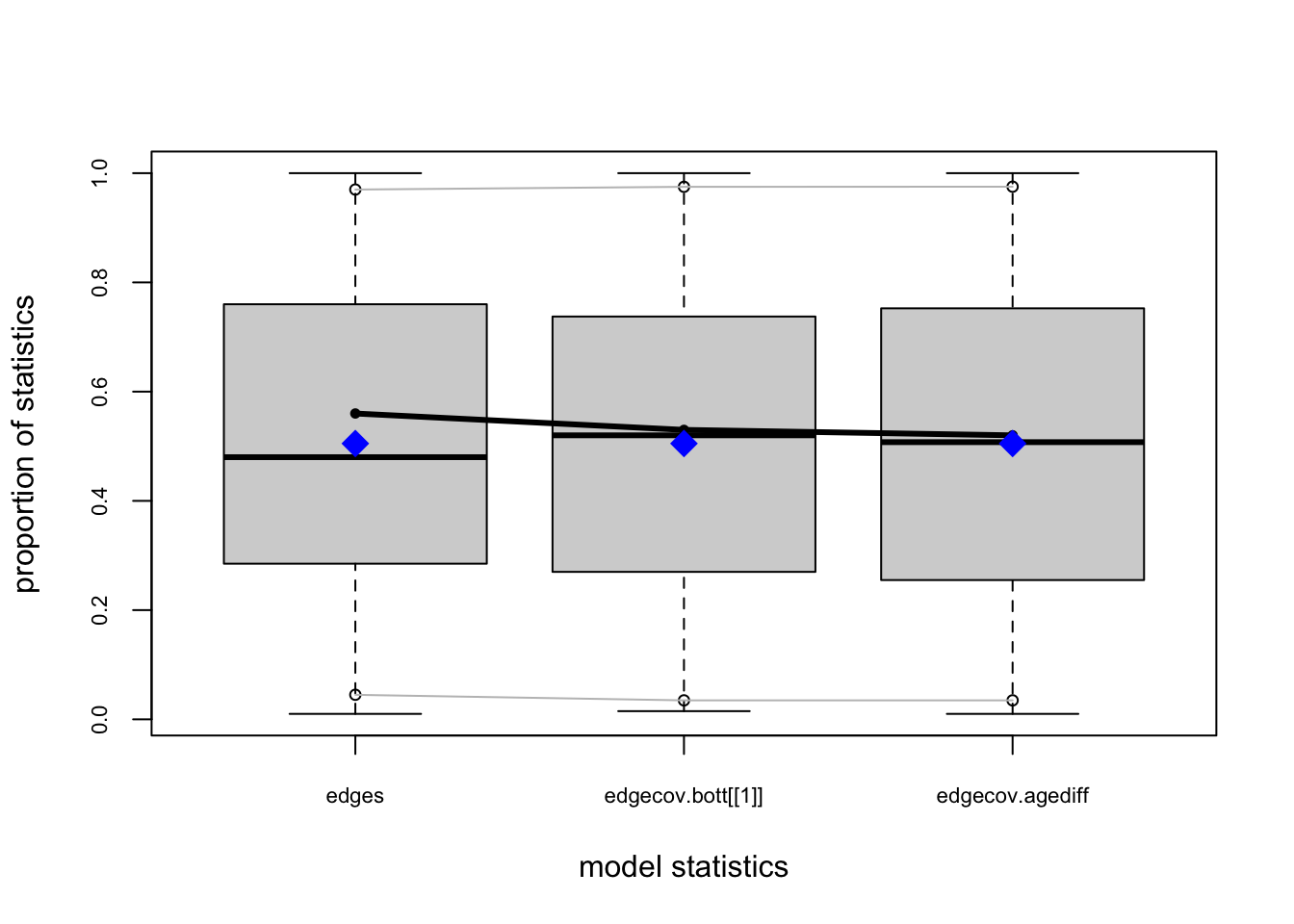
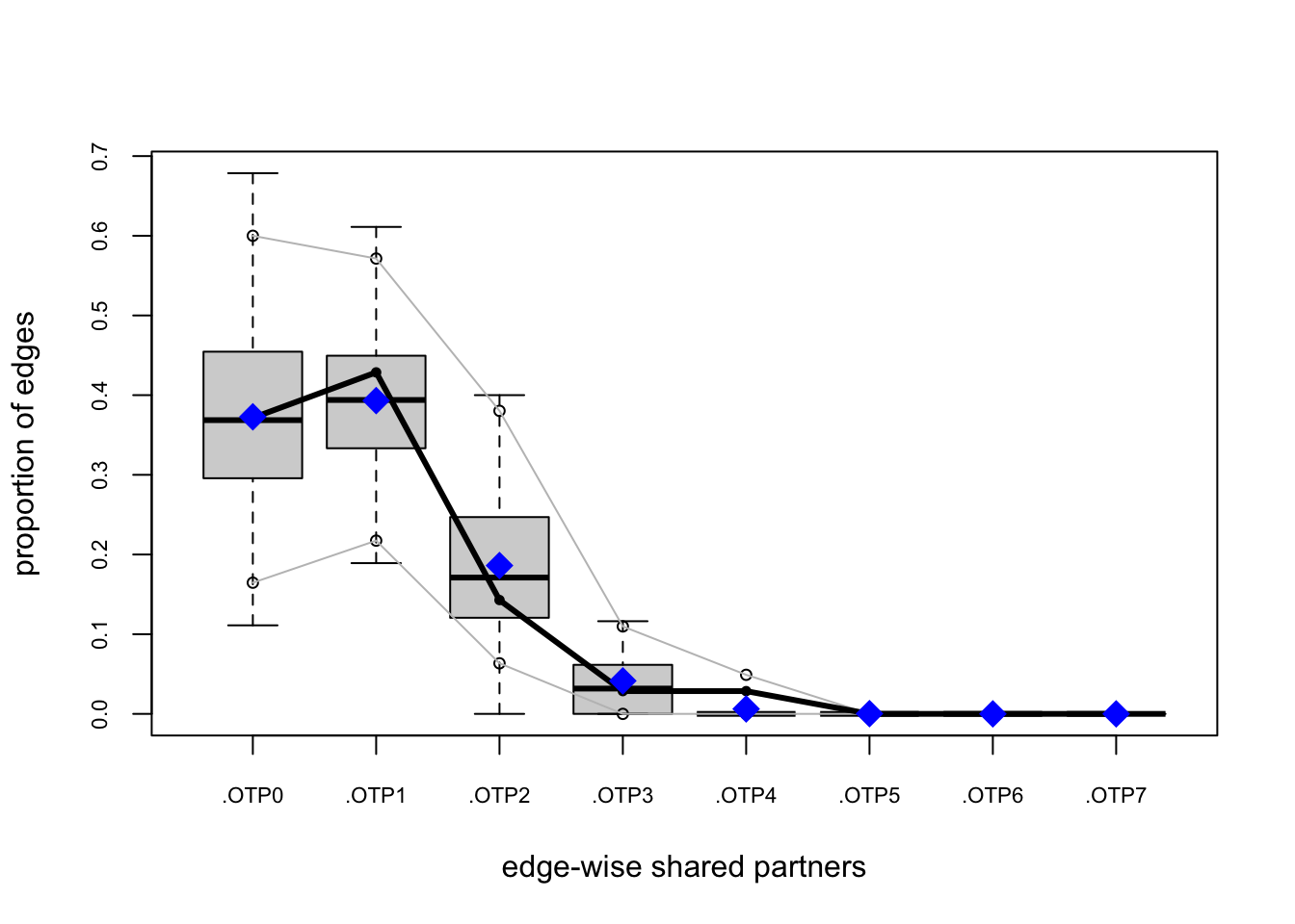
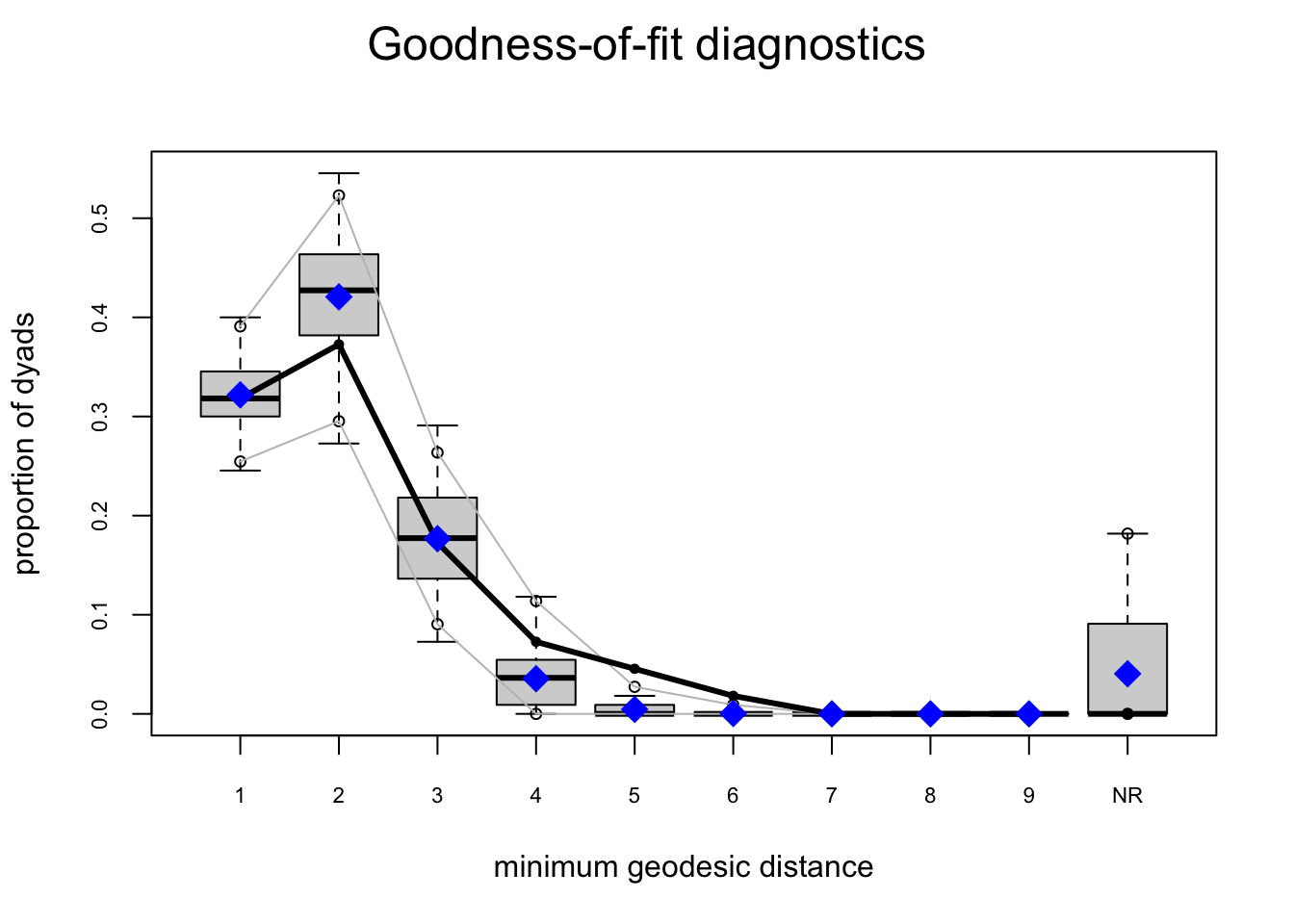
The model-fit looks pretty solid.
Our observed statistics fall within the range of the simulated values, there are no small \(p\)-values, and our plots show no major red flags.
5.15 Loglinear Models
library(foreign)
nhsls <- read.dta("data/nhsls.dta")
is.f <- nhsls$gender=="female"
fnhsls <- nhsls[is.f,]
## it's a big data set so clean up
rm(nhsls)
## check out distribution of ethnicities in women and their last partners
table(fnhsls$ethnic)
white, non-hisp. black, non-hisp.         hispanic asian/pacif (nh)
            1338              342              184               30
natam/alask (nh)          refusal               dk          missing
27 0 0 0 table(fnhsls$sprace1)
   white    black hispanic    asian    other  refusal       dk  missing
    1194      281      137       13       40        0        0        0
Construct a two-way table which is useful for developing intuitions. We also need counts of the cross-classified partnerships for constructing the data frame we use for the generalized linear models.
sextab <- with(fnhsls, table(ethnic,sprace1))
sextab <- sextab[1:5,1:5]
dimnames(sextab)[[1]] <- c("white","black","hispanic","asian","other")
dimnames(sextab)[[2]] <- c("white","black","hispanic","asian","other")
sextab
sprace1
ethnic white black hispanic asian other
white 1131 12 16 3 15
black 5 268 5 0 0
hispanic 39 1 115 0 3
asian 12 0 0 10 4
other 7 0 1 0 18We can see that the great majority of partnerships involve white women and men. The tendency for ethnically concordant-partnerships is also evident as the largest values in any given row/column always lie along the diagonal. For this sample, it appears that hispanic women and hispanic men are the most “versatile,” having the largest fraction of ethnically-discordant partnerships (though the majority of Asian women’s partnerships are actually discordant, which could be another measure of versatility).
We need a data frame on which we can do the analysis.
partners <- as.numeric(c( sextab[1,],sextab[2,],sextab[3,],sextab[4,],sextab[5,] ))
men <- rep( c("white", "black", "hispanic","asian", "other"), 5)
women <- rep( c("white", "black", "hispanic","asian", "other"), c(5,5,5,5,5))
## could also have done it using expand.grid()
## but this provides more control
Generate variables to specify uniform and differential homophily.
## uniform homophily
uh <- as.numeric(women == men)
## differential homophily
dh <- matrix(0, nr=25, nc=5)
r <- which(uh == 1)
for(c in 1:5) dh[r[c],c] <- 1
colnames(dh) <- c("ww","bb","hh","aa","oo")
Assemble the data frame. We will explicitly coerce our vectors men and women into factors. R will do this automatically when we use them as variables in our loglinear models, but it will change the order to be alphabetical. By explicitly specifying the factors, we can control the order.
women <- factor(women, levels=c("white", "black", "hispanic","asian", "other"))
men <- factor(men, levels=c("white", "black", "hispanic","asian", "other"))
## put it all together
pframe <- data.frame(women, men, partners, uh, dh)
head(pframe)
women men partners uh ww bb hh aa oo
1 white white 1131 1 1 0 0 0 0
2 white black 12 0 0 0 0 0 0
3 white hispanic 16 0 0 0 0 0 0
4 white asian 3 0 0 0 0 0 0
5 white other 15 0 0 0 0 0 0
6 black white 5 0 0 0 0 0 0Set the contrasts to something that makes sense for a loglinear model. Then we are set to specify some models. The first one that we should always consider is the independence model. In this model, the rows and columns have independent effects, as the name suggests. For example,
options(contrasts=c("contr.sum", "contr.poly"))
out.ind <- glm(partners ~ women + men, family = poisson, data = pframe)
summary(out.ind)
Call:
glm(formula = partners ~ women + men, family = poisson, data = pframe)

Coefficients:
            Estimate Std. Error z value Pr(>|z|)
(Intercept)  2.21729    0.08631  25.689   <2e-16 ***
women1       2.21530    0.06339  34.950   <2e-16 ***
women2       0.77219    0.07527  10.258   <2e-16 ***
women3       0.20717    0.08547   2.424   0.0154 *
women4      -1.59733    0.16305  -9.797   <2e-16 ***
men1         2.30562    0.07103  32.460   <2e-16 ***
men2         0.85891    0.08172  10.511   <2e-16 ***
men3         0.14054    0.09446   1.488   0.1368
men4        -2.21450    0.22509  -9.838   <2e-16 ***
---
Signif. codes:  0 '***' 0.001 '**' 0.01 '*' 0.05 '.' 0.1 ' ' 1

(Dispersion parameter for poisson family taken to be 1)

    Null deviance: 6819.0  on 24  degrees of freedom
Residual deviance: 1991.4  on 16  degrees of freedom
AIC: 2088.6

Number of Fisher Scoring iterations: 7
## test exactly how bad the model fit is
1 - pchisq(out.ind$deviance,out.ind$df.residual)[1] 0Pretty bad.
At the other end of the spectrum of models is the saturation model.
out.sat <- glm(partners ~ women*men, family = poisson, data = pframe)
summary(out.sat)
Call:
glm(formula = partners ~ women * men, family = poisson, data = pframe)

Coefficients:
             Estimate Std. Error z value Pr(>|z|)
(Intercept)    -4.988  12153.492   0.000    1.000
women1          8.207  12153.492   0.001    0.999
women2         -2.971  27941.706   0.000    1.000
women3          2.029  21545.838   0.000    1.000
women4         -3.498  27941.706   0.000    1.000
men1            8.335  12153.492   0.001    0.999
men2           -3.118  27941.706   0.000    1.000
men3            1.953  21545.838   0.000    1.000
men4           -8.913  33124.835   0.000    1.000
women1:men1    -4.523  12153.492   0.000    1.000
women2:men1     1.234  27941.706   0.000    1.000
women3:men1    -1.712  21545.838   0.000    1.000
women4:men1     2.636  27941.706   0.000    1.000
women1:men2     2.384  27941.706   0.000    1.000
women2:men2    16.668  37600.139   0.000    1.000
women3:men2     6.077  33124.835   0.000    1.000
women4:men2   -12.698  78495.268   0.000    1.000
women1:men3    -2.399  21545.838   0.000    1.000
women2:men3     7.616  33124.835   0.000    1.000
women3:men3     5.751  27941.706   0.000    1.000
women4:men3   -17.769  76452.543   0.000    1.000
women1:men4     6.793  33124.835   0.000    1.000
women2:men4    -7.430  80486.166   0.000    1.000
women3:men4   -12.430  78495.268   0.000    1.000
women4:men4    19.702  41596.710   0.000    1.000

(Dispersion parameter for poisson family taken to be 1)

    Null deviance: 6.8190e+03  on 24  degrees of freedom
Residual deviance: 3.9047e-10  on  0  degrees of freedom
AIC: 129.15

Number of Fisher Scoring iterations: 22
Now we can fit some more interesting models. First, let’s look at the uniform homophily model, which includes main effects for women and men as well as a term for the ethnically-concordant partnerships.
out.uh <- glm(partners ~ women + men + uh, family = poisson, data = pframe)
1 - pchisq(out.uh$deviance,out.uh$df.residual)
[1] 2.066902e-12Looking at the residual deviance, it is a great improvement on the independence model. However, it is still not a good model as we can see from the very low \(p\)-value associated with the chi-square statistic on the residual deviance.
out.dh <- glm(partners ~ women + men + ww + bb + hh + aa + oo, family = poisson, data = pframe)
1 - pchisq(out.dh$deviance,out.dh$df.residual)
[1] 0.01132291