When we first read a graph into R, it is generally a good idea to explore it a bit to get a sense of its overall properties. The best place to start is with the graph summary summary. We can use Padgett’s data on Florentine marriages to explore the analysis of graphs using igraph.
The summary of our graph provides a great deal of information, even if it is a bit terse. The first piece of information is that it is, in fact, an igraph object. Following iGraph indicator, we get a one-to-four letter code indicating what type of graph it is. For the Florentine marriage graph, it is of type UN--, which means that it is undirected (U) and named (N). If our graph was weighted, there would be a third letter W and if it were bipartite, the fourth letter would be B. As gflo is neither weighted nor bipartite, the code is only two letters, UN. Following this two-letter code, we get a summary of the number of vertices and edges in the graph, +16 20. There are 16 vertices and 20 edges in gflo. Finally, we see that there is one attribute contained in the graph, + attr: name (v/c). This means that there is a vertex attribute (v) called “name” which is of type character (c).
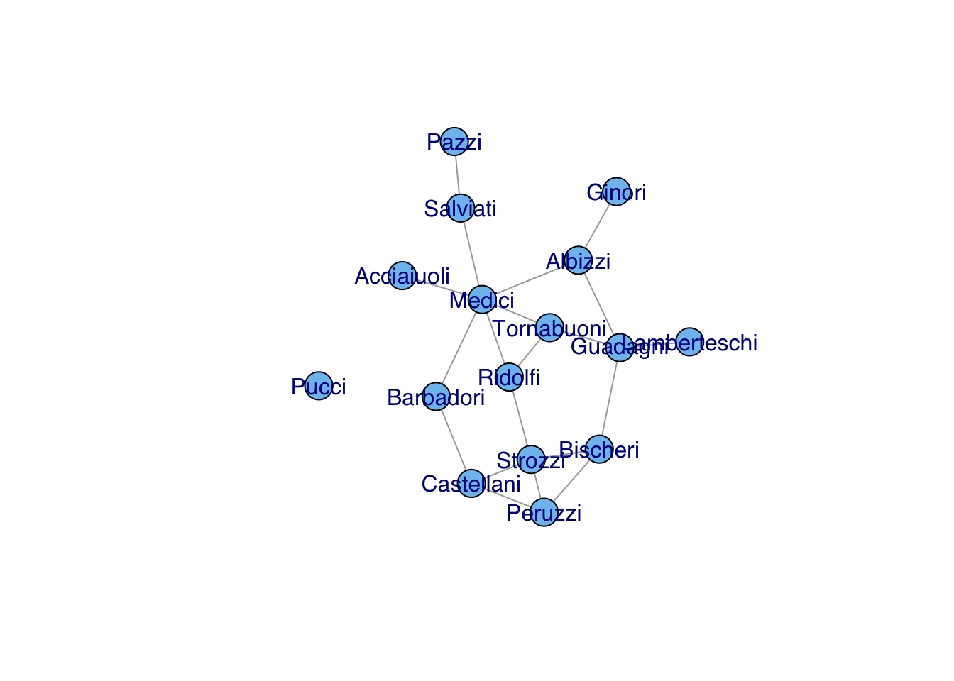
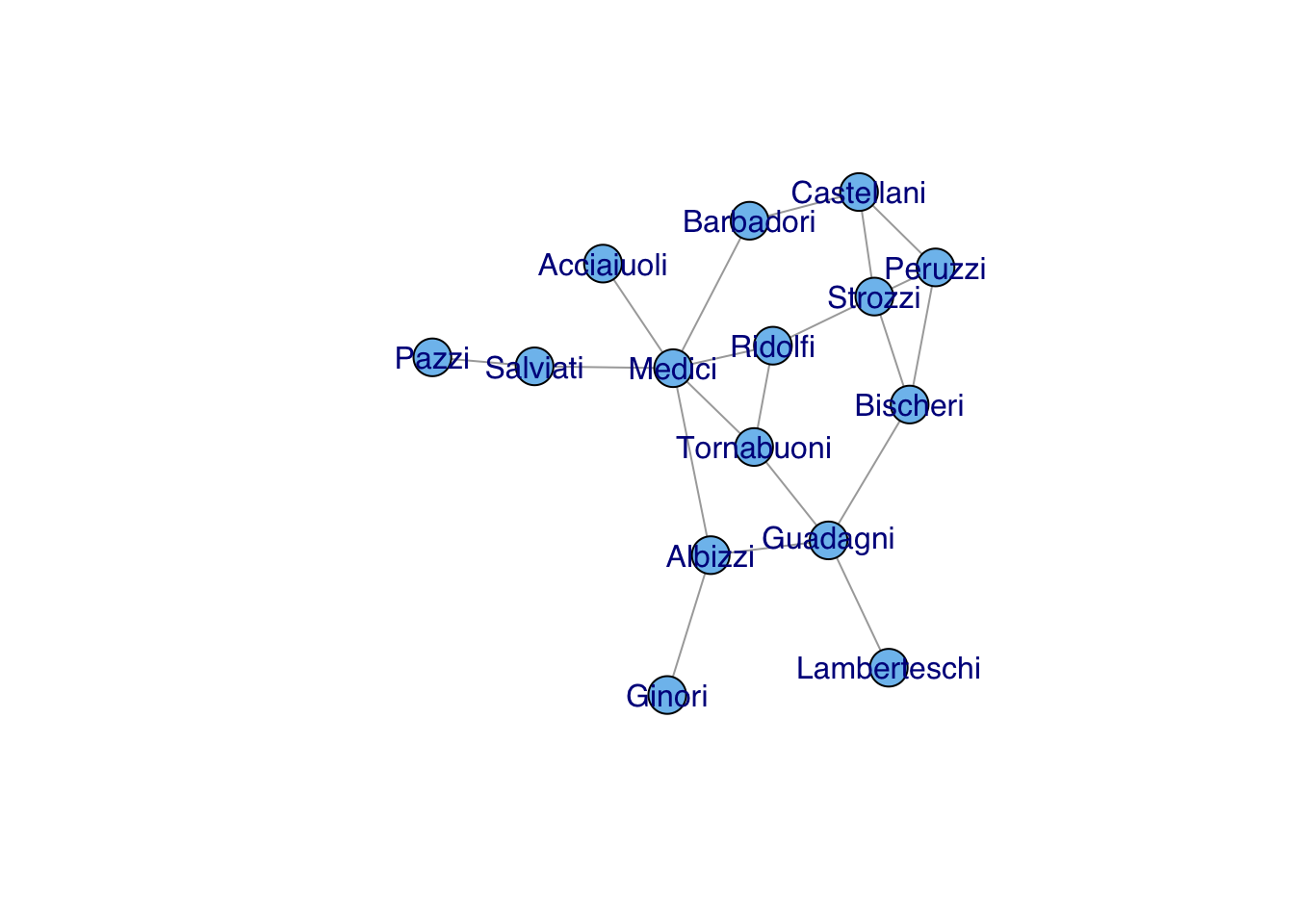
Given that there are a reasonably small number of vertices and (especially) edges, another good idea to to visualize the graph. In general, it is always a good idea to do this. However, if the graph is really big and has lots of edges, the visualization may take some time so you shouldn’t do it casually. For the Florentine marriages, we have only 16 vertices and 20 edges, so plotting is simple.
One of the first things that we discover when we visualize the Florentine marriage network is that one family, Pucci, is an isolate. There were no marriage ties between the Puccis and any of the other 15 families in Padgett’s sample.
Because the graph is so small, it’s easy to see that Pucci is an isolate. In other cases, it may not be so obvious. There are a number of things we can do to study the overall connectedness of a graph. The first is to ask whether the graph is, in fact, connected. For a graph \(\mathcal{G}\) to be connected, there must be a path between all vertices in \(\mathcal{G}\). If the graph is not connected, we might want to know how many distinct components there are. A component is a maximally connected subgraph of a graph (i.e., a path exists between all vertices in the subgraph). We can find the components of our graph using the somewhat unfortunately named igraph function clusters(). The name is unfortunate because “cluster” has many meanings in both network analysis and beyond, but we work with the function names available to us.
We can see that gflo is not connected (since we know from visual inspection that Pucci is an isolate). There are two components in gflo: the main component that includes 15 of the 16 families and then a component of one (Pucci), also known as an isolate.
Knowing that the graph is not connected, we can use the command decompose.graph() to extract the elements. In this case, we really only care about the first component, since the second of the two components is simply an isolate.
gflo1 <-decompose(gflo)[[1]]## could also do this: gflo1 <- induced_subgraph(gflo, subcomponent(gflo,1))is_connected(gflo1)
The number of unordered pairs of vertices in a graph of size \(n\) is \(n(n-1)/2\). This means that the density of edges in a graph is simply given by the ratio of the number of observed edges to the number of possible edges, \(2e/n(n-1)\), where \(e\) is the number of edges in the graph.
## note we're working with the matrix, not the graph object heren <-dim(flo)[1]2*sum(apply(flo,1,sum)/2)/(n*(n-1))
[1] 0.1666667
Here, we summed along the rows of the matrix and then summed the resulting vector to get the number of elements in the sociomatrix. We then divided by two since each marriage is represented twice in the sociomatrix (since it is an undirected relation). Taking out the Pucci isolate, we get a slightly different density. We can use the igraph function graph.density() to reassure ourselves that this is, in fact, the right value.
n <- n-12*sum(apply(flo,1,sum)/2)/(n*(n-1))
[1] 0.1904762
graph.density(gflo1)
Warning: `graph.density()` was deprecated in igraph 2.0.0.
ℹ Please use `edge_density()` instead.
[1] 0.1904762
4.1 The Different Flavors of Centrality
In his classic essay, Freeman (1978) lays out the different notions of centrality:
degree centrality
captures the idea that individuals with many contacts are central to a structure. This measure is calculated simply as the degree of the individual actor.
closeness centrality
captures the idea that a central actor will be close to many other actors in the network. Closeness is measured by the geodesics between actor \(i\) and all others
betweenness centrality
captures the idea that high-centrality individuals should be on the shortest paths between other pairs of actors in a network. The betweenness of actor \(i\) is simply the fraction of all geodesics in the graph on which \(i\) falls.
4.1.1 Degree
For non-directed graphs, degree centrality of vertex \(i\) is simply the sum of edges incident to \(v_i\):
Note that while we call this a “centrality” measure, it is simply the degree of node \(i\) This observation gets the fundamental confounding of degree-based and centrality-based measures of social structure discussed in Salathé and Jones (2010). Sometimes this measure will be standardized by the size of the graph \(n\): \(C'_D(v_i) = d(v_i)/(n-1)\), where we subtract one from the size of the graph to account for the actor itself.
4.1.2 Closeness
For non-directed graphs, closeness centrality of vertex \(i\) is the inverse of the sum of geodesics between \(v_i\) and \(v_j,~~j\neq i\):
where \(d(v_i, v_j)\) is the distance (measured as the minimum distance or geodesic) between vertices \(i\) and \(j\). Note that if any \(j\) is not reachable from \(i\), \(C_C(v_i)=0\) since the distance between \(i\) and \(j\) is infinite! This means that we often want to restrict our measurements of centrality to connected components of a graph. To standardize, we multiply by \(n-1\), the number of vertices not including \(i\): \(C'_C(v_i) = (n-1) C_C(v_i)\).
4.1.3 Betweenness
For non-directed graphs, betweenness centrality of vertex \(i\) is the fraction of all geodesics in the graph on which \(i\) lies:
where \(g_{jk}\) is the number of geodesics linking actors \(j\) and \(k\) and \(g_{jk}(v_i)\) is the number of geodesics linking actors \(j\) and \(k\) that contain actor \(i\). It can be standardized by dividing by the number of pairs of actors not including \(i\), \((n-1)(n-2)/2\): \(C'_B(v_i) = C_B(v_i)/[(n-1)(n-2)/2]\).
Another notion of centrality is that a central person is someone who knows people who know a lot of people. This idea can be captured using a measure known as information centrality. The calculation of information centrality is a bit more complicated than for the other three measures and requires some linear algebra. Start with the sociomatrix \(\mathbf{X}\). From this, we calculate an intermediate matrix \(\mathbf{A}\). For a binary relation, \(a_{ij}=0\) if \(x_{ij}=1\) and \(a_{ij}=1\) if \(x_{ij}=0\) for \(i \neq j\) (that is, the non-diagonal elements of \(\mathbf{A}\) are the complements of their values in \(\mathbf{X}\)). The diagonal elements of \(\mathbf{A}\) (\(a_{ii}\)) are simply the degree of vertex \(i\) plus one, \(a_{ii} = d(v_i)+1\). Once we have \(\mathbf{A}\), we invert it yielding a new matrix \(\mathbf{C}=\mathbf{A}^{-1}\). We then calculate \(T\), the trace of \(\mathbf{C}\), which is simply the sum of its diagonal elements and \(R\) which is one of the row sums of \(\mathbf{C}\) (they are all the same). Information centrality is then simply
\[ C_I(v_i) = \frac{1}{d(v_i) + (T - 2R)/n)}, \]
where, as usual, \(d(v_i)\) is the degree of vertex \(i\) and \(n\) is the size of the graph.
There is no implementation of information centrality in igraph. This can be calculated either in the package sna or in my function infocentral.R. This function takes a sociomatrix as its only argument. It assumes that the matrix is binary.
infocentral <-function(X){## assumes binary relation k <-dim(X)[1] A <-matrix(as.numeric(!X),nr=k,nc=k)diag(A) <-apply(X,1,sum)+1 C <-solve(A) T <-sum(diag(C)) R <-apply(C,1,sum)[1] ic <-1/(diag(C) + (T -2*R)/k)return(ic)}
4.1.4 Eigenvalue Centrality
Yet another approach to centrality was suggested by Bonacich (1972) He suggests that the eigenvectors of the sociomatrix are a fruitful way of thinking about centrality. As with information centrality, the eigenvector approach captures the idea that central people will have well-connected alters but that the relative importance of these alters falls off with distance from ego. While the eigenvector (preferably the dominant one) of the sociomatrix is an excellent measure of centrality, the metric Bonacich (1987) suggests is actually a bit more complex:
where \(\alpha\) is a parameter, \(\beta\) measures the extent to which an actor’s status is a function of the statuses of its alters decay of influence from the focal actor, \(\mathbf{I}\) is an identity matrix of the same rank as the sociomatrix \(\mathbf{X}\), and \(\mathbf{1}\) is a column vector of ones.
The size of \(\beta\) determines the degree to which Bonacich centrality is a measure of local or global centrality. When \(\beta=0\), only an actor’s direct ties are taken into account – Bonacich centrality becomes proportional to degree centrality. However, when \(\beta>0\), an actor’s alters’ ties are also taken into account. The larger the value of \(\beta\), the more distant ties will matter. It is also possible for \(\beta\) to be less than zero. In this case, being connected to powerful alters who themselves have many alters negatively affects an actor’s status. This seemingly odd situation captures the effect observed in bargaining experiments performed on networks by Cook et al. (1983), where an individual’s ability to negotiate a favorable outcome is lessened when he or she must bargain with powerful, well-connected alters.
4.1.5 Comparing Centralities
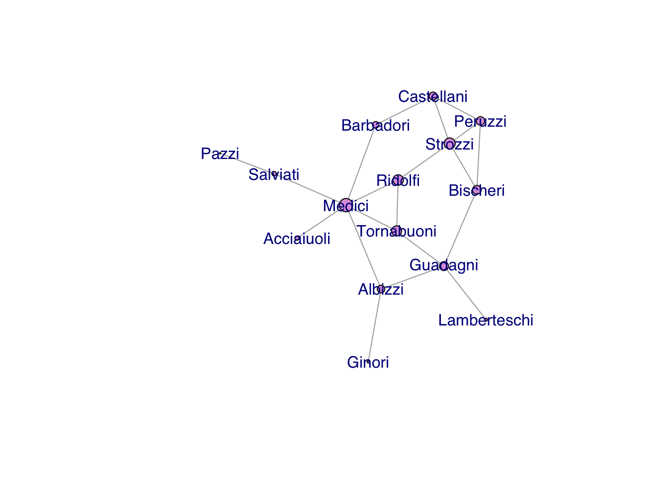
Consider the centrality measures on Padgett’s Florentine marriage data. For these analyses, we will take out the Pucci family since they are an isolate. For the standard centrality measures discussed by Freeman, Pucci will have a score of zero. Information and eigenvalue centrality only work on connected graphs.
# need a matrix# remove Pucciflo1 <- flo[-12,-12]ic <-infocentral(flo1)CP <-abs(power_centrality(gflo1))CE <-eigen_centrality(gflo1)$vectorflo_measures <-cbind(CD=degree(gflo1),CB=round(betweenness(gflo1),1),CC=round(closeness(gflo1),2),CI=round(ic,2),CP=round(CP,2),CE=round(CE,2))dimnames(flo_measures)[[1]] <-dimnames(flo1)[[1]]flo_measures
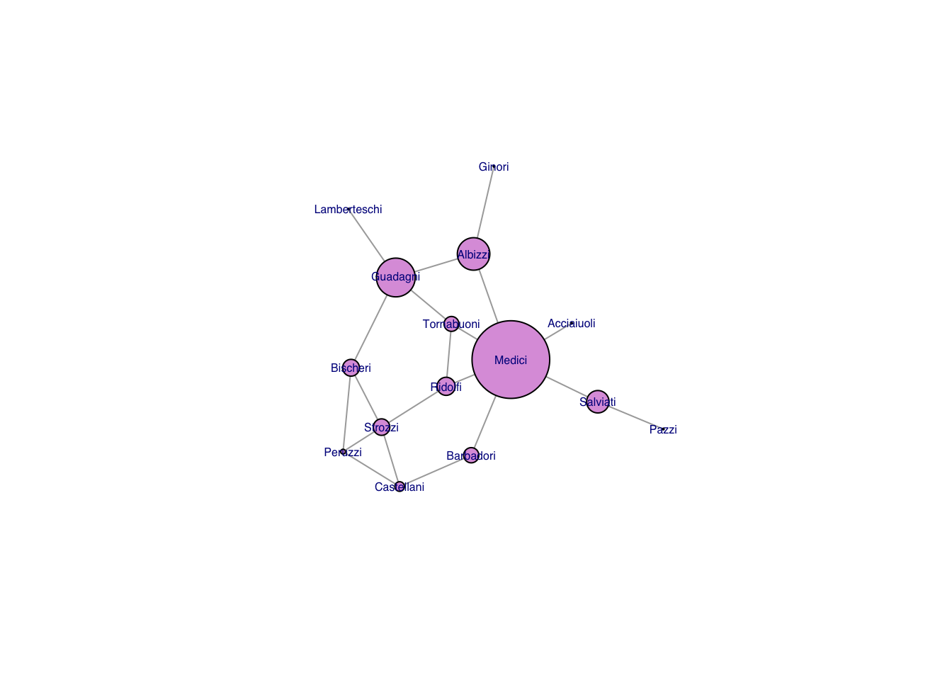
While centrality measures capture different notions of centrality, power, prestige, etc., they are generally fairly highly correlated. This said, some measures can be quite divergent. We can see this with eigenvalue centralities of the Florentine families. The Medici are clearly central to this marriage network. However, because they are so dominant, their alters do not have as many connections as they do. As a result, the Medici have a low eigenvalue centrality, but the Albizzi do quite well.
## correlation matrix of the centralitiescor(flo_measures)
            CD         CB        CC        CI          CP         CE
CD  1.00000000 0.84392220 0.7463380 0.9207909 -0.02813901 0.92473505
CB  0.84392220 1.00000000 0.6592939 0.7143692  0.01003666 0.66445276
CC  0.74633802 0.65929385 1.0000000 0.8238569  0.12584573 0.83955267
CI  0.92079092 0.71436925 0.8238569 1.0000000  0.14762599 0.97762806
CP -0.02813901 0.01003666 0.1258457 0.1476260  1.00000000 0.06943349
CE  0.92473505 0.66445276 0.8395527 0.9776281  0.06943349 1.00000000
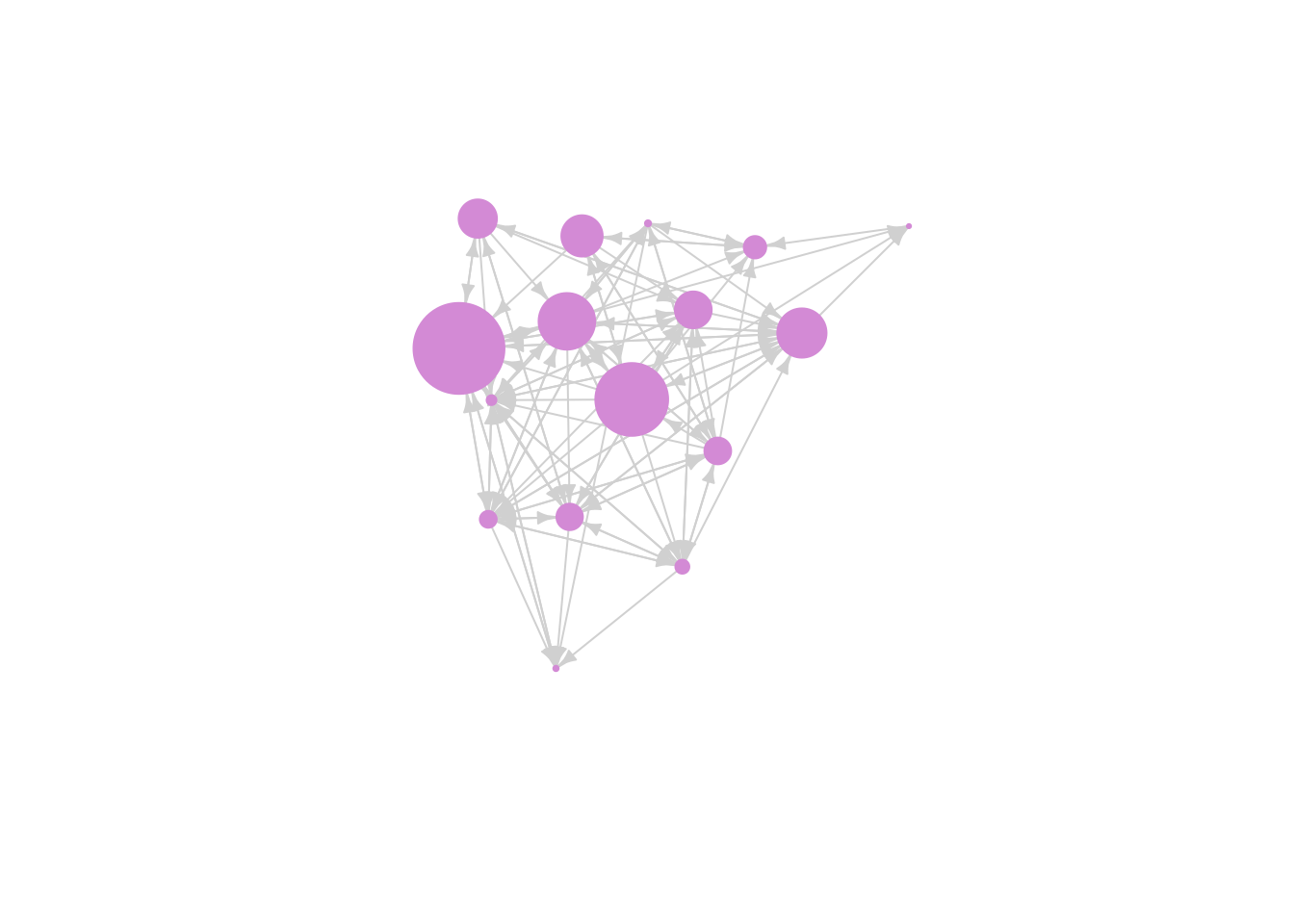
## vertex size proportional to eigenvalue centralityplot(gflo1, vertex.size=flo_measures[,"CE"]*10, vertex.color="plum",vertex.label.family="Helvetica")
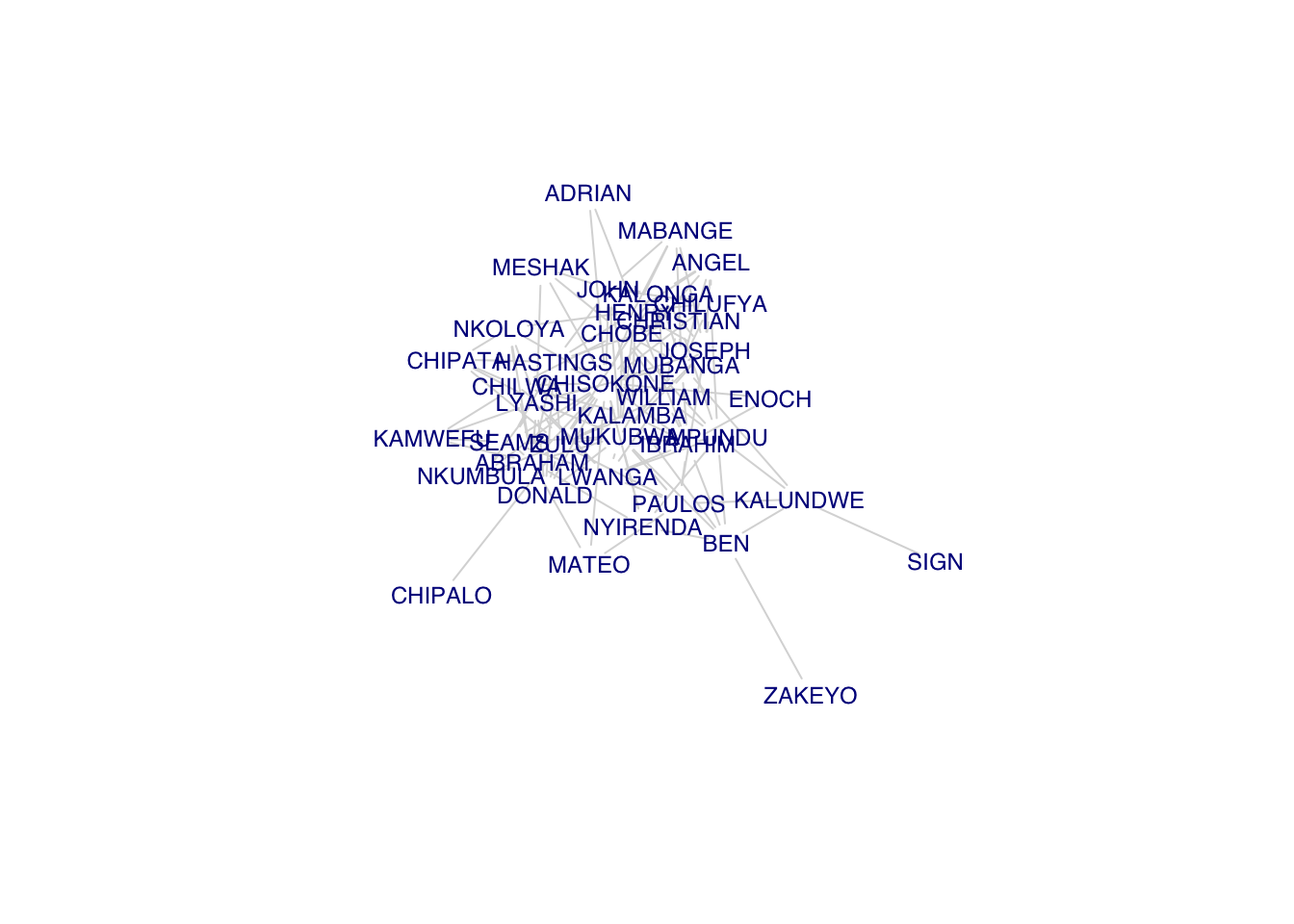
We can redo our comparative analysis of centralities with Kapferer’s tailor shop.
A <-as.matrix(read.table("data/kapferer-tailorshop1.txt", header=TRUE, row.names=1))G <-graph_from_adjacency_matrix(A, mode="undirected", diag=FALSE)plot(G,vertex.shape="none", vertex.label.cex=0.75, vertex.label.family="Helvetica", edge.color=grey(0.85))
Calculate the centralities.
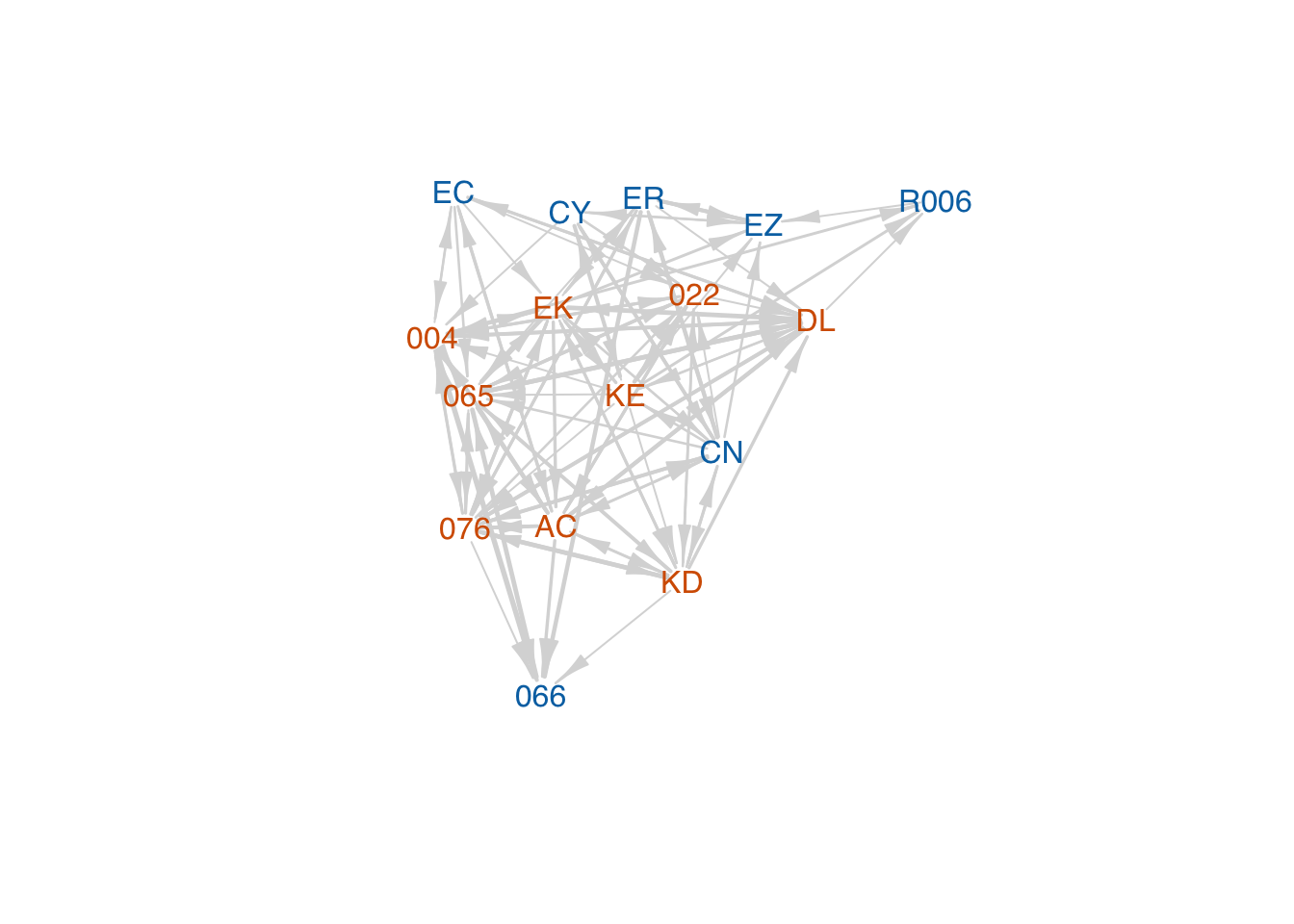
c <-infocentral(A)CP <-abs(power_centrality(G))CE <-eigen_centrality(G)$vectorkap_measures <-cbind(CD=degree(G),CB=round(betweenness(G),1),CC=round(closeness(G),2),CI=round(c,2),CP=round(CP,2),CE=round(CE,2))dimnames(kap_measures)[[1]] <-dimnames(A)[[1]]kap_measures
It is somewhat surprising that the individual with the highest betweenness is 004, who is somewhat peripheral to the core.
Bonacich, Phillip. 1972. “Factoring and Weighting Approaches to Status Scores and Clique Identification.”The Journal of Mathematical Sociology 2 (1): 113–20. https://doi.org/10.1080/0022250X.1972.9989806.
Cook, Karen S., Richard M. Emerson, Mary R. Gillmore, and Toshio Yamagishi. 1983. “The Distribution of Power in Exchange Networks: Theory and Experimental Results.”American Journal of Sociology 89 (2): 275–305. https://doi.org/10.1086/227866.
Salathé, M., and J. H. Jones. 2010. “Dynamics and Control of Diseases in Networks with Community Structure.”PLoS Computational Biology 6 (4): e1000736. https://doi.org/10.1371/journal.pcbi.1000736.