Uncertainty Breaks Intertemporal Choice and Cost-Benefit Analysis
Suppose we have some measured variable which we assume follows a normal distribution with unknown mean and variance. Using Bayesian reasoning, it is straightforward (though tedious) to derive the posterior distribution of both the unknown mean and variance (this is known as the joint posterior distribution). However, we’re typically primarily interested in the mean in applications and relegate variance to the status of a “nuisance parameter,” necessary for estimation of the quantities of interest but not generally of direct interest itself. One therefore typically focuses on the marginal distribution for the mean by averaging over the uncertainty in the variance. This leads to the interpretation of the posterior distribution as being a mixture of normals with the same mean, conditional on the variance – i.e., we essentially overlay different bell-shaped normal curves with different heights and breadths but all centered at the same point.
With some standard assumptions about our prior information on this measurement, guess what the resulting distribution is? If you’ve been paying attention and haven’t been lulled to sleep, you probably guessed Student’s \(t\)-distribution! This is the classical result that is used in a \(t\)-test for comparing two means with unknown variance. The best estimate of the mean is the sample mean, and its standard deviation is given by the standard error. How spread out a \(t\)-distribution is depends on the number of degrees of freedom it has. This is essentially just the number of observations that are used to estimate the distribution. If you have fewer data, you have fewer degrees of freedom and a shorter, wider distribution. The fewer the degrees of freedom, the greater the uncertainty.
Geweke (2001) made this observation. He used a simple Bayesian conjugate model for a normal mean. If the variance of the distribution is known, the posterior is simply another normal with variance scaled by the sample size. However, if the variance is also unknown, the marginal posterior distribution is \(t\). The heavy tails come from the fact that you have to integrate the normal distribution for the mean over the uncertainty in variance. If you have a finite number of trials in which to learn, you end up with heavy tails. The moment-generating function for the \(t\) distribution does not exist and this means that expected utility is not well-defined.
So what? As we discussed above, the Student-\(t\) distribution is known as a fat-tailed or heavy-tailed distribution. This essentially means that there is non-negligible probability of extreme outcomes. More technically, we can say that a random variable is heavy-tailed if and only if its moment generating function \(M(s)\) is infinite for all \(s > 0\). We can also say that a random variable \(X\) is heavy-tailed if the log of the probability of \(x\) as \(x \rightarrow \infty\) decays sub-linearly (Nair, Wierman, and Zwart 2022). This latter condition captures the idea that there will be non-negligible probabilities potentially associated with extreme values when a random variable has a heavy-tailed distribution.
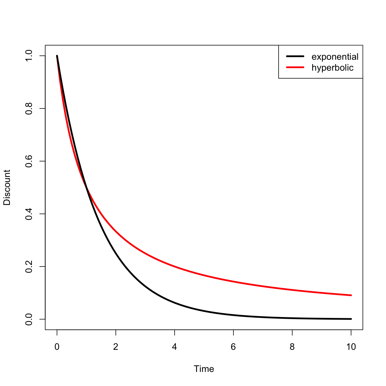
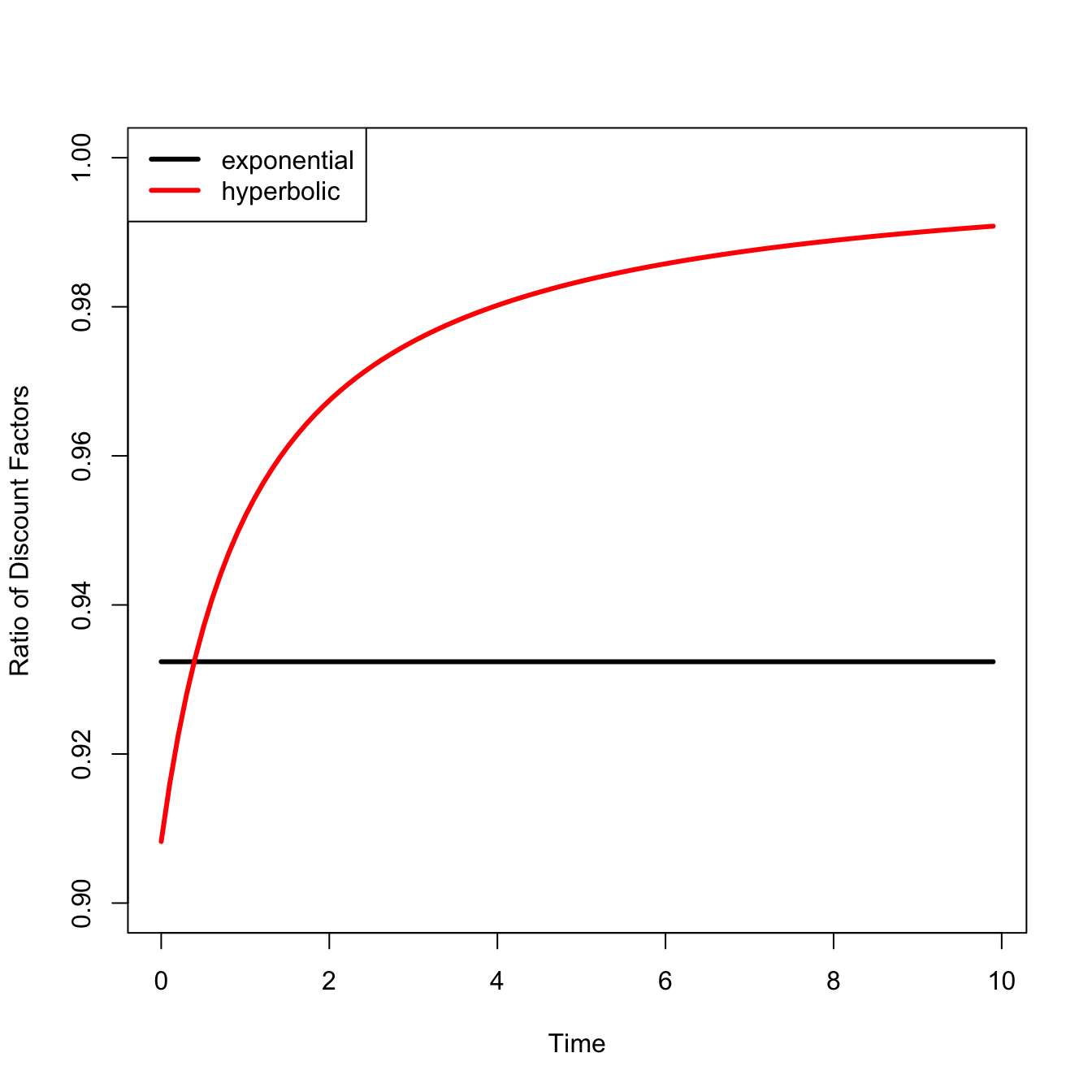
We do a cost-benefit analysis (CBA). Discount the future benefits. A funny thing happens when we calculate the expected utility of investing in climate mitigation when the distribution of future disutility is a fat-tailed. The benefit to averting the worst outcomes is essentially infinite. So we can discount the future as much as we want in order to favor the immediate. Ain’t no discounting infinity tho.
M. L. Weitzman (2009) argues that the logic that leads from structural uncertainty to heavy-tailed distributions of environmental outcomes naturally leads to a precautionary principle. Weitzman also notes that his so-called “Dismal Theorem” makes positing an ad hoc additional of ambiguity aversion to the theory of decision-making under risk unnecessary.
Integrate that text with the more technical bits:
The natural conclusion from the CBA is that, given the fat tail of outcomes-of-global-warming distribution, is that strong action to mitigate the future effects of this looming problem is clearly rational.
Notes that the expected moment, \(E[M] = \beta\; E[\exp(-\eta Y)]\), is the amount of present consumption the agent would be willing to give up in the present period to obtain one extra sure unit of consumption in the future. \(Y\) is the log of “reduced-form consumption that has been adjusted for welfare by subtracting out all damages from climate change” (\(C\)).
\(\beta\) is the time-preference parameter (\(\delta = -\log(\beta)\)) is the instantaneous rate of pure time preference) in the ‘stochastic discount factor’ or ‘pricing kernel’ ” (quotes in original)
\[M[C] = \beta \frac{U'(C)}{U'(1)} = \beta \exp(- \eta Y)\]
\(E[M]\) is a shadow price for discounting future costs and benefits.
Letting \(y\) represent a realization of the random variable \(Y\), and \(f(y)\) denoting the PDF of \(Y\) (this is the expected stochastic discount factor),
\[E[M] = \beta \int_{-\infty}^{\infty} e^{-\eta y} f(y) dy\]
\(E[M]\) is the Laplace-transform or moment-generating function of \(f(y)\). This is convenient since it means that the expected stochastic discount factor has the same properties as the moment-generating function of the PDF of \(f(y)\).
The MGF of a t-distribution is infinite. This is true for any fat tail distribution (Nair, Wierman, and Zwart 2022).
Without well-defined moments of the distribution, you cannot do standard cost-benefit analysis. That “expected” in expected utility theory refers to the first moment of a distribution!
the \(t\)-distribution arises from a compounding a normal distribution with known mean and variances given by an inverse-gamma distribution (which is a standard distribution for unknown variance). When you marginalize (i.e., average over) this unknown variance, the resulting distribution of \(t\).
Denote the data used for calculating the posterior distribution \(y\), the parameters of this distribution \(\theta\), and new data not yet collected as \(\tilde{y}\). The posterior predictive distribution of \(\tilde{y}\) given \(y\) can be written as:
\[
p(\tilde{y}|y) = \int_{\Theta} p(\tilde{y}|\theta) p(\theta|y) d\theta
\]
That is, we calculate the expectation of \(\tilde{y}\), given the posterior distribution \(p(\theta|y)\).
“Something quite extraordinary seems to be happening here, which is crying out for further elucidation! Thousands of applications of EU theory in thousands of articles and books are based on formulas like (5) or (6). Yet when it is acknowledged that s is unknown (with a standard noninformative reference prior) and its value in formula (5) or (6) must instead be inferred as if from a data sample that can be arbitrarily large (but finite), expected marginal utility explodes. The question then naturally arises: What is EU theory trying to tell us when its conclusions for a host of important applications—in CBA, asset pricing, and many other fields of economics—seem so sensitive merely to the recognition that conditioned on finite realized data the distribution implied by the normal is the Student-t?” (p. 8)
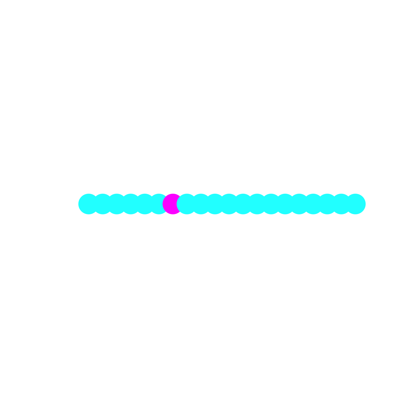
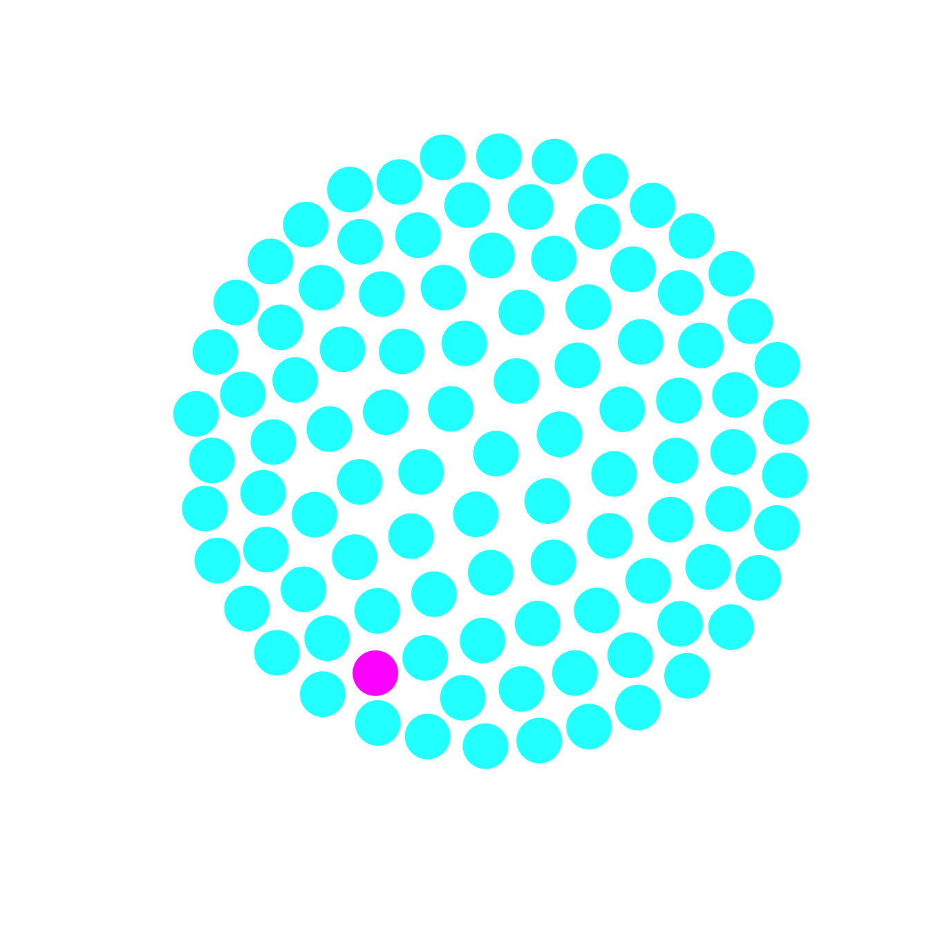
Experience will generally overweight information on the least-consequential part of the outcome distribution. Rare but highly-consequential outcomes are still rare. You are unlikely to experience one in a small sample.
Weitzman’s Dismal Theorem (DT):
\[ \lim_{\lambda \rightarrow \infty} E[M|\lambda]] = +\infty \]
i.e., as the value of statistical life gets large, the shadow price of future consumption becomes infinite.
“No matter how much data-evidence exists—or even can be imagined to exist—DT says that \(E[M|\lambda]\) is always exceedingly sensitive to very large values of \(\lambda\)” (p. 12).
(where \(\lambda\) the statistical-value-of-life-like parameter)
Generalized Ramsey formula for the risk-free interest rate:
\[ r^f = \delta + \eta \mu - \frac{1}{2} \eta^2 s^2 \]
where \(\delta\) is the rate of pure time preference, \(\mu\) is the mean of \(Y\), the log of adjusted consumption), \(\eta\) is the CRRA parameter.
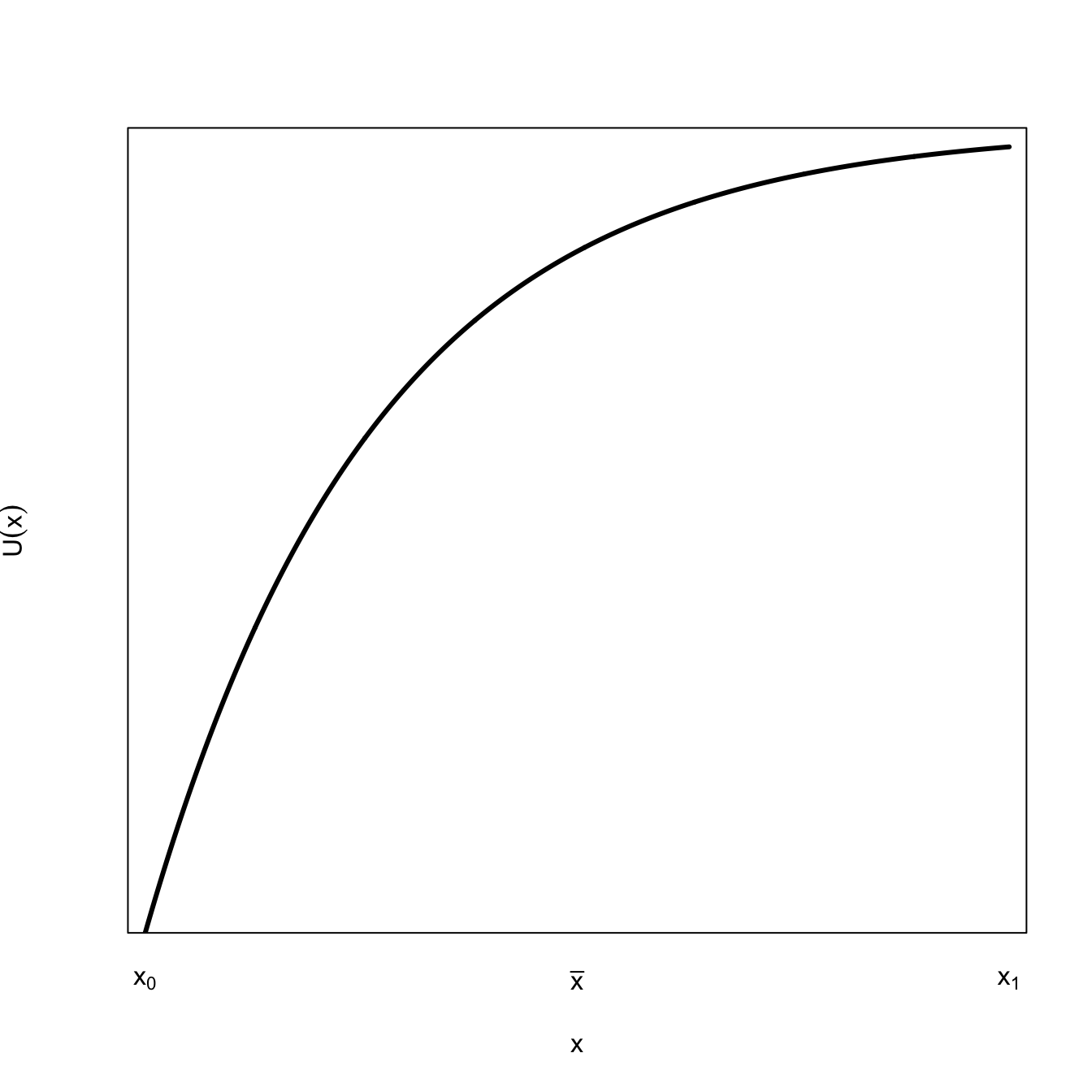
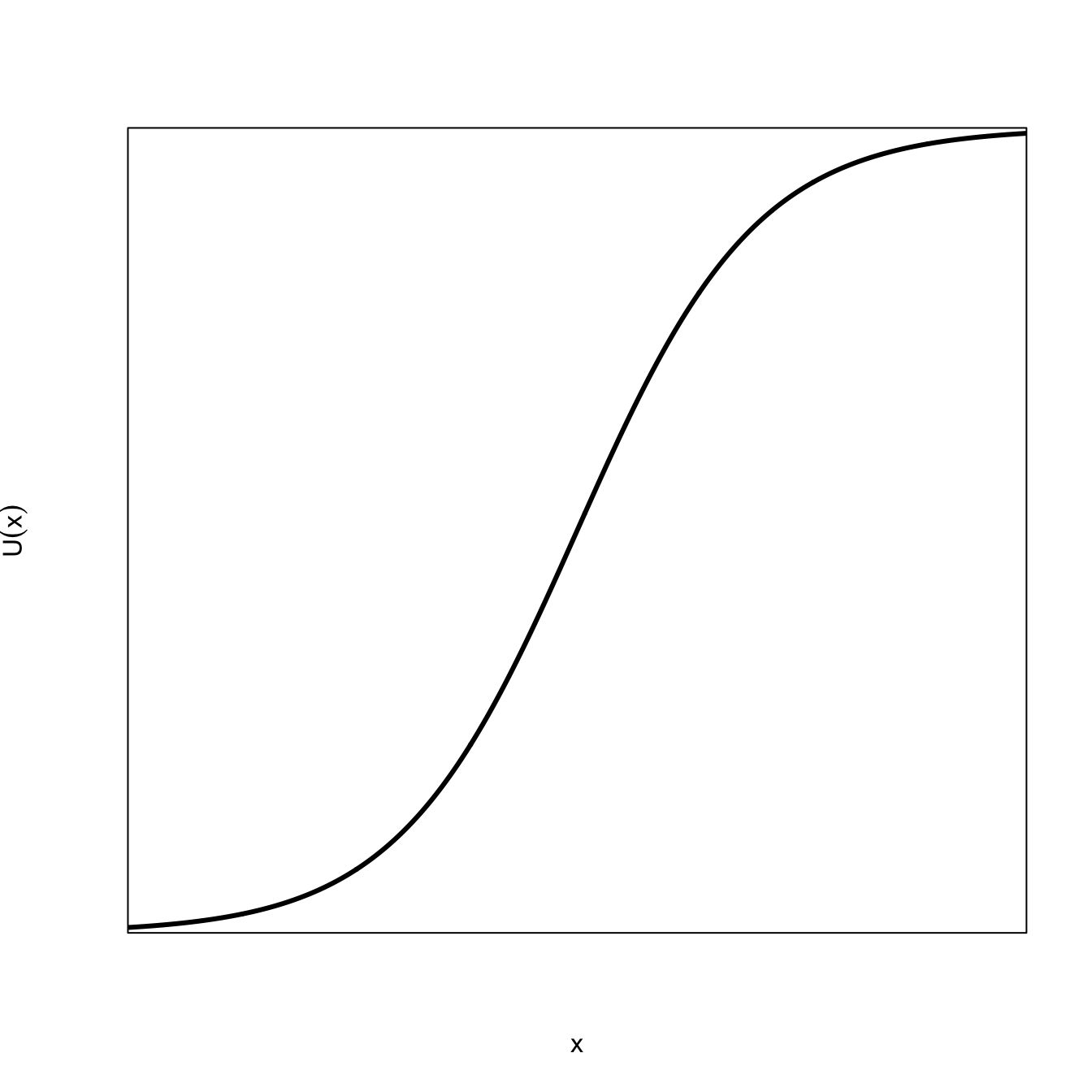
This assumes that utility is CRRA, of course. CRRA means constant relative risk aversion. It is a utility model that is also known as the power utility function or isoelastic utility function. For consumption level \(c\), the CRRA utility is given by:
\[
u(c)= \begin{cases}\frac{c^{1-\eta}-1}{1-\eta} & \eta \geq 0, \eta \neq 1 \\ \ln (c) & \eta=1\end{cases}.
\]
CRRA utility is increasing and concave because \(u'(c ) = c^{-\eta}\) The index of relative aversion (\(R\)) to intertemporal inequality is constant, and is equal to \(\eta\).
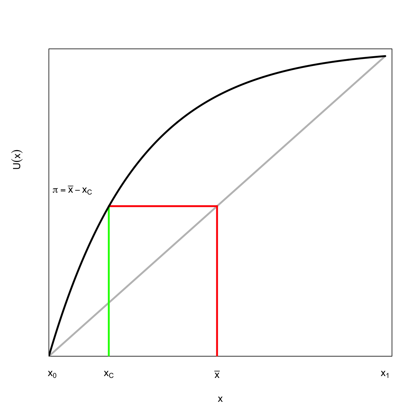
Gollier (2013) explains that the key question is “What is the maximum reduction \(k\) of current consumption that you are ready to sacrifice, or invest, to increase future consumption by 1 dollar?”
The power utility form makes big assumption that \(k\) only on the growth rate and not on the initial absolute level of consumption. Moreover, Gollier (2013) notes that a power utility is inappropriate when there is the possibility of ruin. For example, it suggests that marginal utility tends to infinity when \(c\) approaches zero. This means that if there was some future state of the world where consumption approached zero, someone using a CRRA utility function would be ready to sacrifice almost 100% of their current wealth to increase wealth in this future state by one dollar. This means that we should be very cautious about any strong statements about extreme futures made using CRRA.