x <- seq(-10,10,length=1000)
plot(x,dunif(x,-10,10), type="n", axes=FALSE, frame=TRUE,
     xlab="Outcome", ylab="Probability of Outcome")
arrows(-10,0.05,10,0.05,code=3, lwd=2)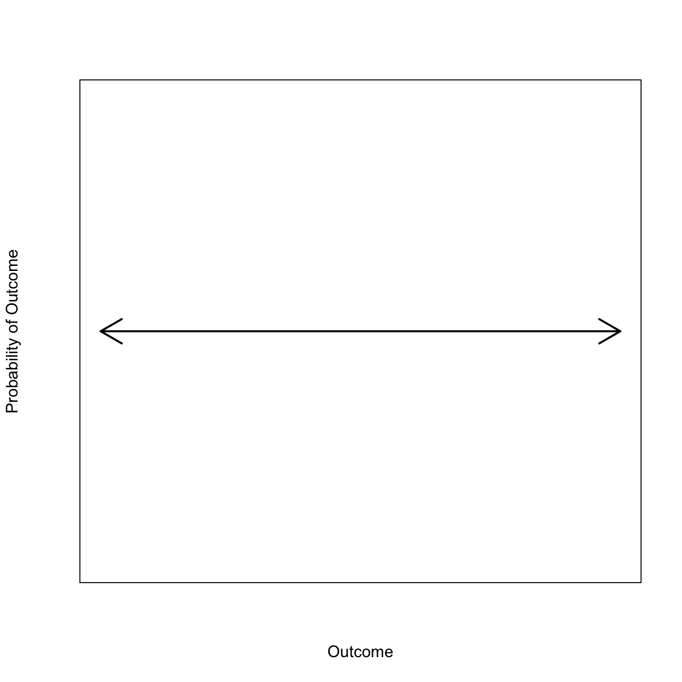
I have been pretty obsessed with risk for a while now. My interest in formal risk management was piqued when I began thinking about life-history strategies for variable environments. The formal analysis of risk seemed like a pretty big absence from life history theory, particularly in the literature pertaining to the evolution of human life histories. I first articulated some of these ideas in a review I wrote for Current Biology back in 2011. A more recent articulation of this work as it relates to life histories is this paper with Mike Price, where we show that fitness maximizers employ nonlinear probability weighting to decisions (with life-history consequences) under risk. This may sound a bit obscure, but it’s important because nonlinear probability weighting is one of the hallmarks of economic irrationality as seen by the Biases and Heuristics school of behavioral economics. Nonlinear probability weighting may not be rational from the orthodox axiomatic perspective, but it will keep you from going extinct! Better alive and “irrational” than extinct and consistent with some dude’s (arbitrary) axioms.
Without getting too far into the weeds, the standard approach to decision-making under risk involves choosing the “prospect” (i.e., a course of action with a variable payoff) with the greatest expected utility. That is, for all the prospects you’re choosing between, sum up the products of the utility of each possible outcome and its associated probability (that’s what an expectation is) and pick the one that’s biggest. If we’re thinking about evolution, we would substitute the word “strategy” for “prospect” and, of course, “fitness” for “utility,” but the decision criterion remains the same. We now just imagine that it’s natural selection that is “choosing” in the sense that individuals who employ strategies with the highest expected fitness will come to dominate the population.
As Mike’s an my paper suggests, it might actually be more complicated than that.
More recently, I’ve done a bit of a re-think on things and have come to the conclusion that the real action for understanding human evolution—and the future of human adaptation—is uncertainty. Colloquially, risk and uncertainty sound similar. They both involve non-deterministic payoffs. But there is a fundamental difference between them that was recognized over a hundred years ago in the publications of two of history’s great economists. Both John Maynard Keynes and Frank Wright published major works in 1921. In Risk, Uncertainty, and Profit, Knight neatly summarized the fundamental distinction between risk and uncertainty, “Uncertainty must be taken in a sense radically distinct from the familiar notion of Risk, from which it has never been properly separated…The essential fact is that ‘risk’ means in some cases a quantity susceptible of measurement, while at other times it is something distinctly not of this character; and there are far-reaching and crucial differences in the bearings of the phenomena depending on which of the two is really present and operating…. It will appear that a measurable uncertainty, or ‘risk’ proper, as we shall use the term, is so far different from an unmeasurable one that it is not in effect an uncertainty at all.”
A full articulation of his views of uncertainty would not come from Keynes until the later publication of his better-known, General Theory in 1936, but in his 1921 Treatise on Probability, he did express great skepticism about the usefulness of expectations in rational decision-making. The language he used reflected his unorthodox views on probabilities. In part IV of his Treatise, Keynes wrote “The second difficulty, to which attention is called above, is the neglect of the ‘weights’ of arguments in the conception of ‘mathematical expectation.’ … In the present connection the question comes to this—if two probabilities are equal in degree, ought we, in choosing our course of action, to prefer that one which is based on a greater body of knowledge?” Here, he was really saying essentially the same thing as Knight. If we can’t actually measure the probabilities properly, we can’t use expectations to guide our decisions.
I now have a lot to say about uncertainty and how organisms faced with it might nonetheless make adaptive decisions. I will save this for future posts—and maybe even some peer-reviewed publications? (hope springs eternal). However, for the rest of this post, I will lay out what I think is a pretty heuristic way of thinking about what uncertainty is.
Suppose we have absolute uncertainty over the value of some outcome. That is, we have absolutely no idea what the value could be. What we get is a uniform distribution, which looks like a horizontal line drawn at a height such that the area under it sums to one. If we really have no idea whatsoever what the value can be, then this line goes from minus infinity to infinity and is infinitesimally high.
x <- seq(-10,10,length=1000)
plot(x,dunif(x,-10,10), type="n", axes=FALSE, frame=TRUE,
xlab="Outcome", ylab="Probability of Outcome")
arrows(-10,0.05,10,0.05,code=3, lwd=2)
We gather data to help us estimate the outcome. The more informative the data are that, the more precise our estimate will be. The effect that this has on our probability distribution is as though we were simultaneously pushing up at the most likely value compatible with the data and down on the extremes. Note that failure to observe extreme values is itself information and the more trials you go without observing extreme events, the more your beliefs shift to believe that extremes are rare.
plot(x,dunif(x,-10,10), type="n", axes=FALSE, frame=TRUE,
     xlab="Outcome", ylab="Probability of Outcome")
arrows(-10,0.05,10,0.05,code=3, lwd=2)
arrows(-7,0.051,-7,0.1, col="red", code=1, lwd=2)
arrows(7,0.051,7,0.1, col="red", code=1, lwd=2)
arrows(0,0,0,0.049, col="red", code=2, lwd=2)
##
plot(x,dnorm(x,0,3.5), type="l", lwd=2, axes=FALSE, frame=TRUE,
     yaxs="i", ylim=c(0,0.12),
     xlab="Outcome", ylab="Probability of Outcome")
arrows(-7,0.051,-7,0.1, col="red", code=1, lwd=2)
arrows(7,0.051,7,0.1, col="red", code=1, lwd=2)
arrows(0,0,0,0.049, col="red", code=2, lwd=2)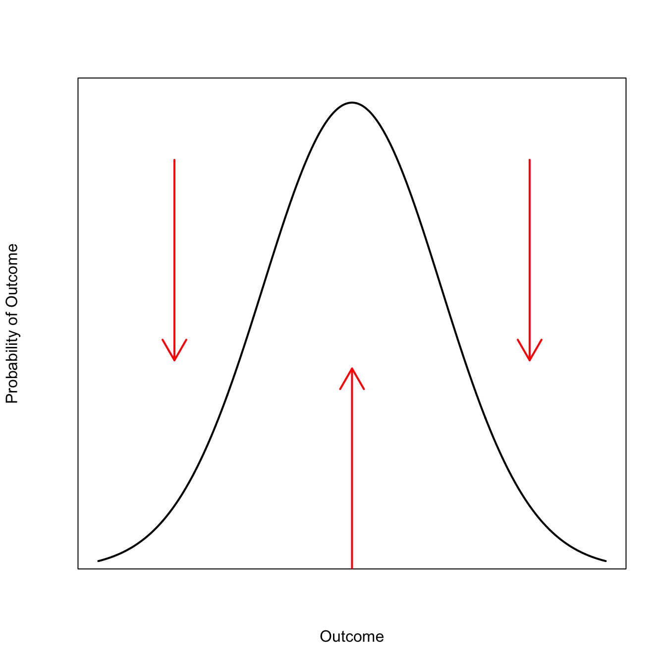
As we keep adding informative observations, our distribution becomes taller and has shorter tails.
plot(x,dnorm(x), type="l", lwd=2, axes=FALSE, frame=TRUE,
     yaxs="i", ylim=c(0,0.42), xlim=c(-10,10),
     xlab="Outcome", ylab="Probability of Outcome")
arrows(-7,0.051,-7,0.1, col="red", code=1, lwd=2)
arrows(7,0.051,7,0.1, col="red", code=1, lwd=2)
arrows(0,0,0,0.049, col="red", code=2, lwd=2)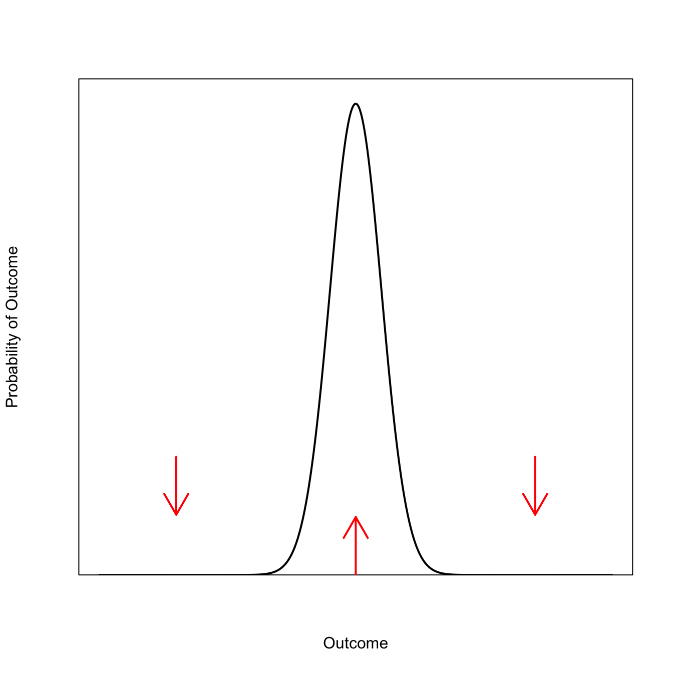
In the limit, if our data were perfectly informative, we would get a point mass on the “true” value of the outcome. This is a magical world that I frankly don’t believe in—diversity is the rule in biology—but it is useful to think of the two limiting cases that bracket our ability to estimate things: complete uncertainty is a horizontal line; complete certainty is a vertical line.
So as we make ourselves less uncertain, we make our probability distribution more vertical around a central point. Returning to the Keynesian perspective on uncertainty, suppose we have an estimate of our outcome, but that we are not at all certain that our probabilities are correct. They have low ‘weights’ in the Keynesian sense. This case is actually nicely formalized in a Bayesian framework when we marginalize, i.e., average our estimates over unknown (nuisance) parameters. The canonical case is estimating a normal mean with unknown variance using the conjugate model. I will save the details for another post, but the punchline is that the distribution of a normal mean with unknown variance under the standard conjugate model is a t-distribution with degrees of freedom equal to the sample size of your data.
This may seem unremarkable. We’ve all done t-tests. The thing is, the t-distribution has some pretty wild properties. Most notable among these is that it is heavy-tailed (or fat-tailed). There is a nice, relatively new text (including full preprint) on heavy-tailed distributions here. Heavy-tailed distributions are one way of thinking about uncertainty.
Again, I will leave the details for a later post, but the upshot is that heavy-tailed distributions break expectations. In a short paper in 2001, John Geweke pointed out the degeneracy of expected utility under heavy-tailed distributions. I don’t think enough people know about this result and I will write much more about it later.
For now, let’s just let is suffice to say that a heavy tail is kind of like adding back that horizontal element to a probability distribution. The tails aren’t really horizontal, but they’re certainly more horizontal than thin-tailed distribution: by definition, the probability of a heavy-tailed variate decays sub-linearly on a log scale (i.e., slower than exponential).
Here’s a comparison of our normal distribution with a low-df t-distribution. While the two distributions are centered on the same point, the t-distribution is less peaked, has wider shoulders, and much heavier tails. We are less certain of our estimate.
plot(x,dnorm(x), type="l", lwd=2, axes=FALSE, frame=TRUE,
     yaxs="i", ylim=c(0,0.42), xlim=c(-10,10),
     xlab="Outcome", ylab="Probability of Outcome")
lines(x,dt(x,df=1), lwd=2, col="red")
The existence of a heavy-tailed distribution means that very large (or very small) values are not impossible. We can compare the tails of a normal distribution and a low-df t-distribution.
plot(x,dnorm(x), type="l", lwd=2, axes=FALSE, frame=TRUE,
     yaxs="i", xaxs="i", ylim=c(0,0.4), xlim=c(0,10),
     xlab="Outcome", ylab="Probability of Outcome")
lines(x,dt(x,df=1), lwd=2, col="red")
abline(h=0.01,lty=3)
axis(1)
axis(2)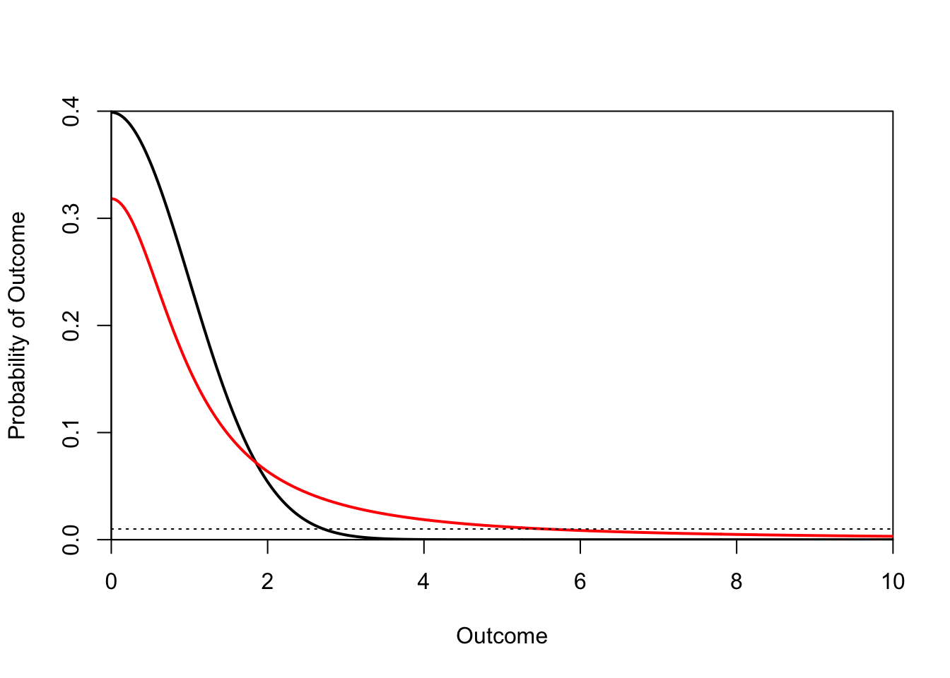
It’s common to refer to extreme events by the number of standard deviations they are from the mean. As the conventional variable name for standard deviation is \(\sigma\) (i.e., the Greek letter sigma), we call something the magnitude of which is two standard deviations away from the mean a \(2\sigma\) event, and so on. From the figure, we can see that while the probability of observing a \(4\sigma\) event is essentially zero for the normal distribution, the probability of a \(6\sigma\) event is approximately 1% (1 year out of 100) for the \(t\) distribution. The probability of a \(9\sigma\) event is 0.5% and of a \(10\sigma\) event is 0.3%. Another way to think about that is that we should expect a \(10\sigma\) event approximately every 300 years or about 12 human generations.
The nonzero probability of these very extreme events causes the variance to blow up. The variance is, in fact, infinite for this distribution (and for \(df=1\), the mean is undefined since a standard t-distribution with one degree of freedom is also a Cauchy (0,1) distribution).
It’s tough to minimize variance when the variance is infinite! It’s also impossible to rank prospects according to their moments (e.g., mean and variance) when the moments aren’t defined.
Organisms (like humans) who face real—or Knightian—uncertainty still need to make decisions. If they can’t choose on the basis of expectations, what do they do? It’s an important question and will be the subject of future posts and (hopefully) forthcoming papers.