On Average

Unpublishable Papers

By any reasonable standard, I am an interdisciplinary scholar. Interdisciplinarity is often held up as being an academic ideal. Honestly, I think of it as a bit more of a curse. I can’t help myself, but the way I think and work frequently lands me in uncomfortable spaces between—and sometimes at odds with—disciplines. This, of course, is why we aspire to interdisciplinarity—because getting out of our comfort zone causes us to question our assumptions and sometimes leads to new insights, new approaches to problems, and new solutions.

It’s not so much the discomfort that makes it a curse, but the simple professional consequence that my interdisciplinarity often leads to writing a category of work that I—only somewhat jokingly—call my unpublishable papers. These papers are unpublishable not (necessarily) because they’re bad. It’s just that there’s no obvious outlet for them (I have a related corpus of work that I could call my unfundable grants).

I’ve decided to bite the bullet and just post some of these here on monkey’s uncle. This first unpublishable post is not a scholarly paper, but an argumentative essay. It’s an argument that I’ve repeatedly lost with editors, but I think it’s important. Students have read versions of this essay in my courses The Uncertain Future of Humanity and The Social Science of Sustainability, where it anchored a whole module of each class.

I originally wrote this essay for the Berggruen Prize Essay Competition. Obviously, I didn’t win the prize. So I had this 10,000-word essay lying around and after licking my wounds for a while (and by “a while,” I mean two years), and a couple rounds of students discussing it, I thought maybe I would try to break it up into a couple smaller essays in the hopes of making something more publishable. This post is that failed effort. I submitted “On Average” to various serious outlets, but there really just aren’t that many places an essay like this could be published even in theory. I mostly heard nothing from the editors. One time, an editor actually wrote me back and gave me a critique straight from his PPE tutorial on expected utility. My response went unanswered and my sense of the unpublishable nature of the essay was strengthened. I am now deeply into the realm of diminishing-marginal-returns to effort on this essay, so I will inaugurate my new series of unpublishable papers and essays here in an effort to at least get the idea out in a somewhat more public forum. Since I face no word limit, I can add some extra material to the stripped-down version I previously circulated. Publishing here also means I can add figures and maybe even a little math if I’m feeling particularly wacky.

The Hidden Choice in Maximizing Expected Value

The staggering recent growth of prediction markets suggests that people must really like betting. Another question altogether is whether we’re any good at it. So, in the spirit of the moment, let’s play a little betting game. Imagine that every week we flip a coin. If it comes up heads, your money doubles; tails, you lose 60% of it. How do you feel about this bet? Do you play or pass? Bear in mind that you are staking your entire bankroll each round. Does that change your choice?

Presumably, the rational way to make your decision is to do the math the way you were taught in high school. On the face of it, this is a fantastic bet. Half the time you double, half the time you keep 40 cents on the dollar. Average it out: (0.5 × 2) + (0.5 × 0.4) = 1.2. This is your expected return. On average, you gain 20% per flip. Forever. Compounded weekly, that expected value makes you a millionaire embarrassingly fast. On a platform like Kalshi or Polymarket, a contract with a documented 20% expected edge, repeatable indefinitely, would be the most important financial discovery of your life.

You may have guessed that there’s a catch. The indefinite 20% return is an expectation. Suppose you took that bet for a year. You would watch your bankroll plummet toward zero. Not in expectation, but in reality; on the timeline where we actually live our lives.

Going broke is essentially mathematically-guaranteed with enough flips, despite the very appealing expected value of this gamble. How can that be? The expected-value calculation isn’t wrong, exactly. It’s just answering the wrong question. The question it addresses is best understood with an example. Assemble a thousand people and endow them with $100 to play our game. On the first flip, about half of them will see their money doubled, while the other half will be down to $40. Take the average bankroll of our thousand players and it will be just about $120. This is an average in “space.” You do the averaging over the possible outcomes, or state space of the gamble. A large collection of people will accurately reflect this space of outcomes. Now pick a single individual out of the thousand. After the first round, she has either $200 or $60. Each round compounds on what happened previously. Within about 50 rounds, she will almost certainly be bankrupt.

The problem is, you don’t care about a summary of the aggregate of many people’s bankroll. You care about what happens to you. As a result, you care about the time average. In a time-averaged condition, a long-enough string of tails ends the game, and once your bankroll hits zero, there is no flip that brings it back. This is what we call an absorbing boundary in the biz. Zero times two is still zero.

Why do we do this weird thing where we substitute this hypothetical aggregate average across the space of possible outcomes rather than the one we actually want across time? Simply put, time averages are hard to calculate. They, er, take time. Moreover, we genuinely want something more general than the specific timeline we’re on because we are betting on the future and the future hasn’t happened yet. The problem is that when you are betting on something that compounds, that is, when your future outcome is a multiplicative function of the present, the space average and the time average almost never the same. Technically, this is known as non-ergodicity.

The physicist Ole Peters has helped to develop a field called Ergodicity Economics. Here is a history of the ideas of ergodicity economics. For the most part, mainstream economists are unimpressed. I am actually quite sympathetic to some of the criticisms. However, I think the ideas are extremely important—probably for quite different reasons that the EE guys. I come to this problem more from the perspective of a population biologist. Where these ideas are particularly important is in the realm of policies related to existential threats, that is, threats that entail the possibility of extinction. This is what motivates my interest.

The Average That Lies, and the One That Doesn’t

Bets are more than just entertainment. A bet involves three things: a stake, an uncertain outcome, and a payoff. In our example, the stake is your bankroll, the uncertain outcome is the coin flip, and the payoff is how your bankroll is modified depending on the outcome of the coin-flip (i.e., doubled or reduced by 60%). Every time we make a decision about a course of action for the future, we make a bet. A farmer makes a bet about what to plant. His stake is the capital he expends on factors such as seed and fertilizer and the labor of planting, weeding, and harvesting. The uncertain outcome is the size and value of the harvest. The payoff is the surplus value he derives from eating his produce or selling it on a market. A high school senior makes a bet on whether she should attend a college where she’s been accepted. The stake is the money she must pay in tuition and the foregone income from the years spent in further schooling. The uncertain outcome is how she does and how well it prepares her for life after college. The payoff is a lifetime of enhanced opportunity and increased earning power. A government makes a bet about policy, such as its future energy policy. The stake is the capital from its treasury (derived, for example, through taxing its citizens). The uncertain outcome is which energy future actually comes to fruition based on technological development, geopolitics, and market forces. The payoff is cheaper and more abundant energy owing to the multiplicative effects of infrastructure and experience.

All of these bets are made in our unique universe, anchored in time. They’re all compounding, though what compounds differs: the farmer’s seed capital, the graduate’s portfolio of acquired capacities, the energy sector’s accumulated experience and falling cost curve. So is there a better measure that we can use to help us decide when we bet on compounding outcomes? It turns out that the standard expectation—or arithmetic mean—is not the only mean we could use. The fact that we use the arithmetic mean is a choice.

What we actually want for that coin-flip bet is called the geometric mean. Instead of adding the outcomes together, you multiply them, then take the root. For our bet, that’s the square root of (2 × 0.4), which is roughly 0.89. Rather than a 20% gain, it’s an 11% loss every single flip, on average, in the only sense of “average” that describes what happens to your actual bankroll over time. The geometric mean isn’t just a variant of the arithmetic mean. Mathematically, it’s tied to compounding. Population biologists use exactly this math to model extinction for the same reason, namely, population growth compounds, and a population that hits zero doesn’t get a do-over. The geometric mean better approximates the thing we care about as individuals anchored in time. If you had employed the geometric mean criterion in our motivating example, you’d have known not to take the bet.

There’s a third average worth knowing. It’s called the harmonic mean, and it is even more allergic to bad outcomes. We calculate it by taking the reciprocal of the average of the reciprocals of our observations. It’s dragged down hard by your smallest values, the way a single catastrophic year dominates a system’s resilience. As with the geometric mean, the harmonic mean would have advised us not to take the repeated weekly bet since it’s value for that bet was even lower at 0.67. The harmonic mean is the tool geneticists use to measure how much genetic diversity a population retains after a bottleneck, because what matters there aren’t the good years, but whether you survived the worst one. In a bad year, a population is likely to lose rare variants and thus diversity. In a good year, an equivalent number of rare variants won’t be spawned through mutation. This is an asymmetry that causes the bad years to dominate.

Of these three means, the arithmetic mean is always biggest. It asks what an average looks like when it’s spread evenly across every possible outcome. It is highly influenced by extreme values. As such, it can hide substantial inequality. The geometric mean measures an average that accounts for the drag on growth that arises from variability. The more variable the elements that you average are, the lower it will be relative to the arithmetic mean. The harmonic mean measures an average weighted to the perspective of the smallest or worst-off in the population. If any of the elements you are averaging is much smaller than the others, this average will be lower still than the geometric and arithmetic means. These are different questions that require different summary measures and lead to different answers.

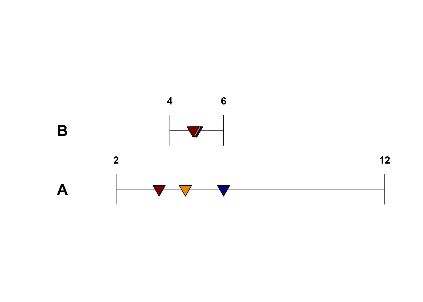
Consider a simple example. We have two lotteries, \(A\) and \(B\). Each lottery has three possible payoffs that are equally likely. For \(A\), these are $12, $4, and $2, and for \(B\), they are $6, $5, and $4. Your bet involves choosing the lottery you would rather play. The expected payoff for \(A\) is $6, while it is $5 for \(B\), so standard expected-value maximization means you pick \(A\). If, on the other hand, we used a geometric-mean criterion, \(B\) would win with a value of $4.93 vs. \(A\)’s $4.58. The preference for \(B\) is even stronger if we use the harmonic mean as our average, with \(B\) at $4.86 and \(A\) all the way down to $3.60. \(A\) is a high-risk/high-gain lottery. It wins if we are comfortable with inequality. The two alternative criteria penalize \(A\) for its inequality (the geometric) or its low minimum payoff (the harmonic).

The following figure shows this graphically. The lines span the values of the respective lotteries (i.e., run from the minimum to the maximum value). Arithmetic means in blue; geometric means in orange; harmonic means in red. The arithmetic mean of lottery \(B\) is less than that of lottery \(A\), while the geometric and harmonic means of \(B\) are both larger than those of \(A\). Because there isn’t much variance in \(B\), the differences between the three means within that lottery are relatively small.

What if the results of this bet were actually consequential? For example, suppose that you needed a minimum of $4 to live. If this were the case, \(B\) is obviously the better choice and the geometric and harmonic means do a better job of picking the better lottery. Including a basement for persistence makes this simple bet an example of an existential risk. When your very existence depends on the winning a bet—or, more likely, not losing it too badly—your preference for variability and inequality in payoffs can very reasonably change. A necessary predicate that is rarely articulated for outcomes like sustainability and human flourishing more generally, is, simply put, persistence. You can’t very well flourish if you’re extinct. In that case, you’ve lost the existential bet. Perhaps we should adjust our preferences accordingly.

Yes, But What About Utility?

The central-casting response to this problem is the one first suggested by Daniel Bernoulli as a solution to cousin Nicholas’s St. Petersburg Paradox. Suppose you have a utility function (and since this is my blog, I can use symbols!), \(u(x)\), where \(x\) is the size of the payoff. Utility always increases as the payoff gets bigger, \(u'(x)>0\), but it does so at a decelerating rate \(u''(x)<0\). These assumptions capture the fact that, in general, more stuff is better than less stuff, but also that getting more stuff when you already have a lot is worth less marginally than when you don’t have much at all (i.e., utility increases more steeply when you’re poor; more slowly when you’re rich). The resulting concave shape of the utility function tends to mute the effects of extreme inequality on calculating expectations. One of the most common utility functions used in both theoretical and practical work is the Constant Relative Risk-Aversion (CRRA) model. When the CRRA parameter is equal to one, it reduces to logarithmic utility.

The expectation of log utility is, in fact, the log of a geometric mean. Since a logarithm is a positive monotone transformation, this gives you the same outcome as if you used a geometric mean. The concavity of the utility function also builds in risk aversion. Play a lottery anywhere on the utility curve: heads, you go up some increment \(\varepsilon\); tails you go down by \(\varepsilon\). Because of the shape of the utility curve, there is an inherent asymmetry to the upside vs. the downside. Because the curve is decelerating (i.e., \(u(x)''<0\)), the upside will increase your utility less than the downside of the bet decreases it. If you can pay a little for certainty, you would do it. This is what it means to be risk-averse in the expected-utility sense.

So, yes, log-utility is an improvement on linearity with respect to both the inequality and risk problems. However, while economists typically employ a utility function, we use the maximization of expected value as a metric in lots of areas beyond economics. Finance and engineering are some obvious examples.

But even if you are pro-utility, as most decision theorists are, there is still a question of aggregation (an expectation is an expectation). You can take an arithmetic, geometric, or harmonic mean of log utility, just as you can the untransformed values. Take two slightly different lotteries: \(a = (2, 4, 16)\) and \(b = (3, 5, 8)\). Lottery \(a\) is high-risk/high-gain; \(b\) is low variance/inequality. Assume a logarithmic utility function. Because of the negative second derivative of \(\log(x)\), you get the presumably desirable property of diminishing marginal utility/risk aversion, so very big values don’t exert too much influence on preferences. But expectations are expectations and the same properties hold. If we employ expected utility, we prefer \(a\) to \(b\) (\(1.617 >1.596\)). If we employ either the geometric or harmonic means, we prefer \(b\) (\(1.386 < 1.543\) and \(1.188 < 1.491\) respectively). Using the arithmetic mean still bakes in a hidden preference for (or, at least, indifference to) inequality and the possibility of extinction. This is, in fact, my fundamental point. We make a lot out of the assumptions of the utility function. The aggregator, not so much. Yet it is massively consequential.

Much of my interest in this area is motivated by existential risk. While we’re talking about utility, it’s useful to briefly talk about the limitations of common utility functions in this specific context. Logarithmic utility is common, but hardly ubiquitous. It tends to be the conventional utility function in macro and growth theory. Another option is CARA (constant absolute risk aversion) or exponential utility. This is the conventional utility function more commonly employed in finance and insurance. Note that CRRA is not useful for existential problems since its value at zero is undefined. This gets at fundamental issues in choice theory like the necessity that utility functions be bounded. As \(\log(0) \rightarrow -\infty\), this means that CRRA is not bounded for questions that involve ruin. Presumably, this why subfields of economics that really care about zeros (i.e., finance, insurance) don’t use it! Maybe we shouldn’t use it for existential problems of the Earth and/or humanity too. This isn’t just idle musing, as CRRA is the commonly-used utility function in environmental economics.

You Already Made a Choice; You Just Didn’t Know It

Here’s my key message: every time an institution—an investment house, a government agency, a foundation deciding how to spend on charitable activities—tells you a course of action is justified because it “maximizes expected value,” they have made a choice about which average matters, and they are very rarely telling you that’s what happened. Indeed, most people frankly don’t even know they’ve done it. The expectation—the arithmetic mean—is often naturalized to be a neutral measure of the universe. It’s not. It’s a human construction and its use in weighing the possible upside of a bet is very much a choice.

The philosophical stance of Expectationalism (the extreme consequence of which is known as Fanaticism) is where this naturalization lives. Fanaticism is the common perspective of many of the well-known effective altruists and Longtermists like Nick Bostrom and Will MacAskill, and I can’t think of a worse foundation for making decisions about the long-term persistence of the human species. The view holds that you should simply maximize expected value—number of people, years of flourishing, whatever your terminal value is. This often comes with an assumption that value is unbounded. In such a case, when you multiply the utility of outcomes by their probabilities and sum, you can get some pretty perverse behavior such as the infamous Pascal’s Mugging. The Fanaticist perspective depends entirely on what I have suggested are the undesirable properties of expected value. If you’re serious about the long-term welfare of humanity, you should use an aggregator that takes extinction seriously.

Note that, as with our toy examples, the expected value is the measure that’s friendliest to long-shot upsides and least bothered by the possibility of ruin. Even if you’re not bothered by ruin (though I think you should be!), it’s also the choice that is least bothered by inequality, even when we slap an interceding concave utility function on the outcomes. It is not the neutral, view-from-nowhere arithmetic it’s generally presented to be. It’s a bet on the value of the big win outweighing the risk of being wiped out, smuggled into a calculation that gives the impression of cool rationality.

Sometimes that bet will be fine. If you’re betting on the Warriors-Lakers game, by all means, bet on your highest expected payoff (though good luck figuring out the relevant probabilities—that’s a subject for another essay). However, when the stakes are a retirement fund, or the persistence of a species, a civilization, or a planet, the question of which average you’re maximizing isn’t a technical footnote you can leave to the actuaries. It’s literally the whole argument. The next time someone argues for a policy solution to some high-stakes problem by citing its expected value, the math may check out. It’s the choice behind which math to use that’s actually worth arguing about.