Novel coronavirus (COVID19) has a quite high estimated R0, with values ranging from around 2.2 to recent extreme estimates in excess of 6. Given such robust values of the reproduction number, we should expect substantial secondary spread beyong the initial epidemic focus in Wuhan. However, it has not spread beyond China (and indeed Wuhan) to the extent that we might expect, given this high reproduction ratio. Kyra Grantz, Jess Metcalf, and Justin Lessler recently suggested that a high degree of transmission heterogeneity might explain this. They calculate that the epidemiological facts are consistent with a model where 80% of infections are caused by 10% of the cases.
This is consistent with our prior knowledge about coronaviruses, namely, that they show quite skewed transmission. That is, coronavirus transmission dynamics are characterized by the presence of super-spreaders. While the presence of super-spreaders is obviously not good, there is an upside. In particular, the presence of a few super-spreaders can drag the expected number of secondary cases (which is what R0 is at the outset of an epidemic) out toward the tail that they define. Now, the estimate of R0 for the various serious coronavirus diseases (e.g., SARS, MERS, COVID19) are reasonably low in the grand scheme of things. The only way you can have super-spreaders (like the man who contracted MERS in Saudi Arabia, traveled back to Korea and generated 186 cases there) and a value of R0 on the order of 1-2 (or even 4-6) is for most people to infect a very small number of new people. The distribution of secondary cases is highly skewed and the mode probably less than one.
The intuition behind Grantz and colleagues’ explanation of the epidemiological facts of COVID19 is that, if we assume that the expected number of secondary cases a person is likely to generate is a feature of their physiology or the circumstances of their infection (i.e., it can be thought of as a trait they take with them) and you pick people at random with respect to this distribution, you are likely to sample mostly people who are not going to generate lots of secondary cases. As a result, the infection chains emanating from them are more likely to die out quickly and the amount of epidemic dispersal will be limited.
This interpretation has a lot in common with the problem of sampling networks. Indeed, it can actually be thought of as a network-sampling problem. It is well known that a random sample of the vertices of a network will lead to a biased sample of the network’s edges, and vice-versa. This is the basis of the famous friendship paradox, first noted by Scott Feld, namely that your friends have more friends than you do. When the degree distribution of a graph is heterogeneous, and your sample is random with respect to vertex, you will likely under-sample the edges of the graph, making the induced subgraph arising from the sampling possibly far less connected than the parent graph.
We’ll construct a network with a negative binomial degree distribution. Mark Handcock and I showed that the heterogeneity of sexual network degree is well-described by a negative binomial and there is a long tradition in epidemiology of thinking about the distribution of secondary cases following a negative binomial.
A straightforward way to create a network with a negative binomial
degree distribution is to generate a vector of gamma random numbers. We
then treat these values as vector of rate parameters for a Poisson
random numbers. The marginal distribution of a Poisson r.v. with
gamma-distributed rate parameter is negative binomial. We’ll aim for
something that is pretty skewed without being too crazy. We can then
construct a network with our fixed (negative binomial) degree sequence
using the igraph function sample_degseq().
library(igraph)
set.seed(8675309)
rates <- rgamma(100, shape=2.5/5, scale=5)
deg <- rpois(100,lambda=rates)
g <- sample_degseq(deg, method="simple")
plot(g, vertex.size=5, vertex.label=NA, vertex.color="skyblue2")
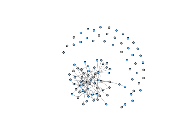
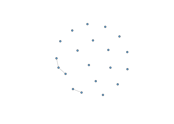
We get a network with a large, strongly-connected component and quite a few isolates. Now we pick a random sample of vertices of our graph.
ss <- sample(1:100, 20, replace=FALSE)
sg <- induced_subgraph(g,vids=ss)
sg <- simplify(sg)
plot(sg, vertex.size=5, vertex.label=NA, vertex.color="skyblue2")
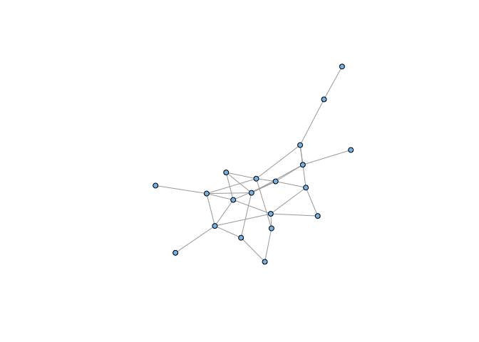
Note that this is not simply a result of taking a small sample of our graph. If we choose correctly, we can recreate a strongly-connected induced subgraph:
sel <- c(3,4,9,16,17,18,19,21,22,25,61,62,64,67,68,85,87,88,92,94)
sg1 <- induced_subgraph(g,vids=sel)
sg1 <- simplify(sg1)
plot(sg1, vertex.size=5, vertex.label=NA, vertex.color="skyblue2")
It’s a bit abstract, but it shouldn’t be too difficult to convince yourself that we could represent the number of potential secondary transmission events from a given case as a network. An epidemic is indicated if the resulting graph is strongly-connected. Sampling the vertices of the heterogeneous network (analogous to moving away from the epidemic focus in Wuhan) leads to an unconnected subgraph and the epidemic dies out.