ERGM predictions and GWESP
Elspeth Ready and Eleanor Power
- Generating ERGM predictions
- Dealing with triangles
- Thinking clearly about ESP
- A worked example
- What about other GW* terms?
- More realistic change statistics
Back to main page.
Generating ERGM predictions
As with other regression methods, ERGMs can be used to predict the probabilities of ties between nodes. Such predictions can be really helpful in interpreting effect sizes and differences between groups of interest in the data.
Calculating predictions from an ERGM is basically the same as for logistic regression: multiply the model coefficients by a set of values, and then transform these log-odds into probabilities. Confidence intervals for point estimates can be generated in the same way.
The key difference between generating predictions for ERGMs and traditional regression methods is in the values that are used to generate the predictions. In ERGMs, the effect of adding any tie to the network on a given network statistic is modelled using the change statistic, which is the difference in the network statistic before and after adding the tie:
Most change statistics are straightforward to calculate. Adding one edge, for example, gives an edge change statistic of 1, and the same for homophily terms: if the tie being modelled is homophilous, the change statistic is simply 1. To calculate predictions, we simply multiply the change statistic for each term by its coefficient, sum all these terms, and take the logistic: , where
is the summation of the model coefficient estimates multiplied by the change statistics for each variable.
Dealing with triangles
As mentioned in our introduction to ERGMs, triangles abound in human social networks. Consequently, ERGMs of human social networks often require a term for transitivity in order to accurately represent the network structure. The current implementation of such terms in statnet is the “Geometrically-Weighted Shared Partnership” family of terms, the most commonly-used of which is GWESP, or “Geometrically-Weighted Edgewise Shared Partnerships.”
Two nodes i and j have an edgewise shared partner when they are connected to each other and both i and j are also connected to a third individual k. If i and j were also connected to node l, then i and j would have two edgewise shared partners. In other words, when nodes have edgewise shared partnerships, they form triangles! Consequently, the GWESP term models the tendency for ties that close triangles to be more likely than ties that do not close triangles. In order to prevent the number of triangles in the network to get out of control, however, the effect of the GWESP term gradually decreases as pairs of individuals have more existing shared partners.
The way that GWESP works can be difficult to understand, and the calculation of the GWESP change statistic is not always straightforward. Here we explain the logic of the GWESP change statistic, in order to clarify the procedure for calculating log-odds and predicted tie probabilities for ERGMs with geometrically-weighted partnership terms, especially GWESP.
The GWESP statistic
The GWESP (Geometrically-Weighted Edgewise Shared Partnerships) statistic, which models triad closure, is calculated as follows (see Hunter 2007):
Where α is the GWESP decay parameter, and pi is the number of actor pairs who have exactly i shared (edgewise) partners. n is the number of nodes in the network; the maximum number of edgewise-shared partners for any pair of nodes in the network is n − 2.
To calculate the change statistic for GWESP, we take this value for the number of edgewise shared partnerships added to the network by the tie you want to predict minus any partnerships that are removed because of the new tie. (When you add ties with shared partnerships, that means you’re removing ties with no shared partnerships!)
Thinking clearly about ESP
Adding one tie has a different effect on the number of edgewise shared partnerships in the network depending on the number of triangles that the tie closes, and the existing number of edgewise shared partnerships that the nodes involved in the triangles already belong to.
Adding a tie that closes no triangles
Fortunately, if a tie being modelled would not close a triangle, then after adding the tie, the nodes will still have the same number of edgewise shared partners, so the GWESP change statistic is zero.
Adding a tie that closes one triangle
The plot below helps illustrate the change in edgewise shared partnerships if a tie closes one triangle, assuming that no nodes in the group have any existing edgewise shared partnerships:
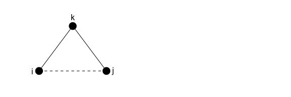
Adding the tie between i and j will add not just one but THREE ties with one edgewise shared partnership to the network (i and j share partner k; i and k share partner j; j and k share partner i). Adding these ties also means “removing” two cases of a tie with zero shared partners (i ↔ k and j ↔ k).
So the change statistic will be:
The first part of the equation above simplifies to 3. We show this with a hypothetical decay parameter of 0.25:
exp(0.25)*(1-(1-exp(-.25))^1)*3
## [1] 3
This is what we expect; the decay parameter doesn’t have any effect when i = 1.
The second part of the change statistic above simplifies to zero:
exp(0.25)*(1-(1-exp(-.25))^0)
## [1] 0
So the change statistic for adding one triangle to the network is 3: three pairs of nodes with one shared edgewise partnership are added to the network when one triangle is closed, again, assuming no existing edgewise shared partnerships among the nodes in the triangle.
Adding a tie that closes one triangle, where nodes already have ESP
The example above assumed that the nodes had no existing edgewise shared partners. What happens if nodes in the triangle to be closed already had some partners in common, as shown in the graph below?
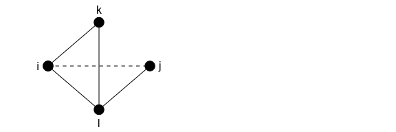
Here, pairs ik, il, and kl already all have one edgewise shared partner. Adding ij will add two instances of one shared partner (for ij and jl), and will increase the ESP of il from one to two. This means that relative to the original graph, there is one additional ESP of one and one ESP of 2.
Now, because we’re adding ties with different numbers of ESP, the summation term in the GWESP statistic will come into the calculation of the change statistic:
Let’s evaluate this with α = 0.25:
exp(0.25) * (((1-(1-exp(-.25))^1)*1) + ((1-(1-exp(-0.25))^2)*1))
## [1] 2.221199
The probability of a tie that closes a triangle where nodes in the triangle already have shared partners is less than the probability of a tie that closes a triangle among nodes that previously had no edgewise shared partners. As the number of existing edgewise shared partners among nodes in the triangle to be closed increases, the change statistic for closing this triangle will continue to decrease. This is the feature of GWESP that allows it to model transitivity without the degeneracy problems of the triangle term!
Adding a tie that closes two triangles
What about adding a tie that closes two triangles? Going back to our original assumption that none of the nodes have any edgewise shared partners, the plot below considers this scenario:
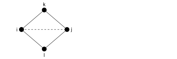
It’s easier to think about this in a table:
| Pair | ESP before adding ij | ESP after adding ij |
|---|---|---|
| ij | 0 | 2 |
| ik | 0 | 1 |
| il | 0 | 1 |
| jk | 0 | 1 |
| jl | 0 | 1 |
| kl | 0 | 0 |
So, closing two triangles adds one tie between nodes with 2 ESP and four ties between nodes with 1 ESP. Four ties between nodes with 0 ESP are “removed.”
The full expression of the change statistic here is:
Which simplifies to:
With hypothetical α = 0.25, this works out to:
4 + (exp(0.25) * ((1-(1-exp(-0.25))^2)))
## [1] 5.221199
A worked example
Calculating log-odds of ties that close triangles
To show how to use the GWESP change statistics to interpret ERGM results, we replicate some of the results presented by Goodreau et al. (2009). They compare the log-odds of ties that close different numbers of triangles (assuming no existing shared partners in the triangles) between students. Their GWESP coefficient is 1.8 and their α value is 0.25.
We’ve already seen that a tie that would close one triangle among nodes with no existing edgewise shared partners would add 1 edgewise shared partnership 3 times, and that consequently, the change statistic for GWESP for closing one triangle is 3. So, the log-odds of a tie that closes one triangle is:
1.8*3
## [1] 5.4
That’s what Goodreau et al. find!
Plugging in our formula from above, a tie that would close two triangles would have a log-odds of:
1.8*(4+(exp(0.25)*(1-(1-exp(-0.25))^2)))
## [1] 9.398159
Goodreau et al. actually present the difference in log-odds between a tie that closes one triangle and one that closes two triangles, so let’s instead express our result as a change statistic from one to two triangles (remembering that closing one triangle adds one edgewise partner three times):
1.8*(4+(exp(0.25)*(1-(1-exp(-0.25))^2)) - 3)
## [1] 3.998159
Voilà! The value they provide is 4.0.
Calculating tie probabilities
If we wish to get predictions for the probability of a tie, we’ll need to consider all of the coefficients and convert the log-odds to probabilities. To illustrate this, we’ll use the model coefficients presented in Table 2 of Goodreau et al. 2009.
We’ll consider three hypothetical ties: one between two male grade 8 students, who are both Asian, but that does not close a triangle; and similar ties that close one or two triangles. For all of these ties, the change statistic will be 1 for the “Edges” term, 2 for “Grade 8” and “Asian” nodecov terms, and 1 for “Grade 8 match,” “Asian match,” and “Sex match” nodematch terms. The GWESP change statistic for the tie that does not close a triangle will be zero. For the tie that closes one triangle, the GWESP change statistic will be 3, as demonstrated above. Finally, for the tie that closes two triangles, the GWESP change statistic will be = 5.221, since α = 0.25 in this model. All other change statistics will be zero, and again, we assume that the nodes in these triangles have no other existing shared partners.
| Model Term | Coefficient | Change stat (no tri) | Change stat (1 tri) | Change stat (2 tri) |
|---|---|---|---|---|
| Edges | -11.188 | 1 | 1 | 1.000 |
| Grade 8 | 0.325 | 2 | 2 | 2.000 |
| Grade 9 | 1.042 | 0 | 0 | 0.000 |
| Grade 10 | 1.636 | 0 | 0 | 0.000 |
| Grade 11 | 1.456 | 0 | 0 | 0.000 |
| Grade 12 | 1.149 | 0 | 0 | 0.000 |
| Black | -0.233 | 0 | 0 | 0.000 |
| Hispanic | 0.743 | 0 | 0 | 0.000 |
| Asian | -0.050 | 2 | 2 | 2.000 |
| Native American | 0.602 | 0 | 0 | 0.000 |
| Other | 0.448 | 0 | 0 | 0.000 |
| Female | 0.168 | 0 | 0 | 0.000 |
| Grade 7 match | 4.142 | 0 | 0 | 0.000 |
| Grade 8 match | 3.648 | 1 | 1 | 1.000 |
| Grade 9 match | 2.165 | 0 | 0 | 0.000 |
| Grade 10 match | 1.094 | 0 | 0 | 0.000 |
| Grade 11 match | 1.552 | 0 | 0 | 0.000 |
| Grade 12 match | 2.226 | 0 | 0 | 0.000 |
| White match | 0.865 | 0 | 0 | 0.000 |
| Black match | 3.166 | 0 | 0 | 0.000 |
| Hispanic match | -0.642 | 0 | 0 | 0.000 |
| Asian match | 2.423 | 1 | 1 | 1.000 |
| Native American match | 0.831 | 0 | 0 | 0.000 |
| Other match | NA | 0 | 0 | 0.000 |
| Sex match | 0.677 | 1 | 1 | 1.000 |
| GWESP | 1.726 | 0 | 3 | 5.221 |
Taking these values, calculate the log-odds for each model term and take the sum:
b1 <- sum(coefs*tie0tri, na.rm=TRUE)
b2 <- sum(coefs*tie1tri, na.rm=TRUE)
b3 <- sum(coefs*tie2tri, na.rm=TRUE)

predsums <- c(b1, b2, b3)

#function to convert summed log-odds to probabilities
logistic <- function(b) {
  exp(b)/(1+exp(b))
}

logistic(predsums)
## [1] 0.02003571 0.78380848 0.99406801
For these hypothetical ties between male Asian Grade 8 students, a tie that closes no triangles has a probability of 0.02, a tie that closes one triangle has a probability of 0.78, and a tie that closes 2 triangles has a probability of 0.99.
What about other GW* terms?
DGWESP
DGWESP terms work according to the same logic as GWESP, but whereas GWESP ignores the directionality of ties within triangles, DGWESP terms account for them. Consequently, only certain types of triangles will count towards the DGWESP statistic.
GWDSP
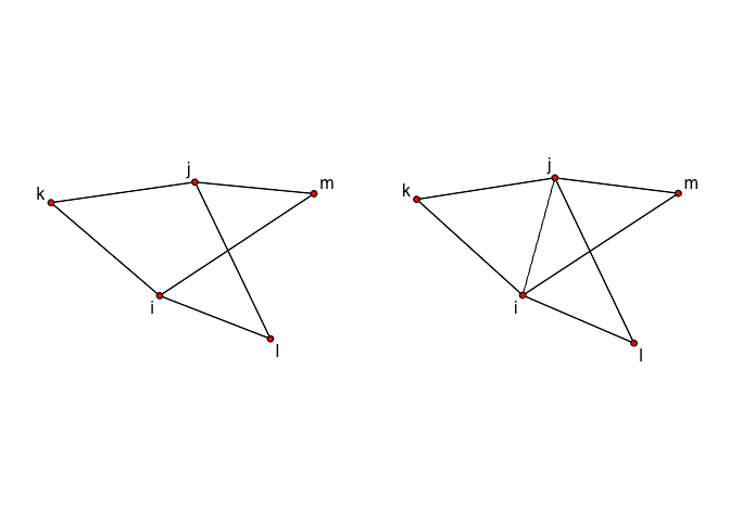
GWDSP counts shared partnerships regardless of whether i and j have a tie. Because it is counted for all dyads with shared partners, even if they are not connected by an edge, figuring out the change statistic for GWDSP is trickier and quickly becomes too many dyads to calculate by hand. To show the process, here we’ll work through an example of closing 3 triangles (assuming no existing triangles among the nodes involved), paying attention not only to changes in ESP, but also to DSP, and we’ll use R to do the calculations for us. We’ll make two versions of the network: one without ij and one with ij.
library(statnet)

#make a toy network
mynet<-network.initialize(5,directed=FALSE)
mynet %v% "vertex.names" <- c("i","j","k","l","m")
mynet["i","k"]<-1
mynet["i","l"]<-1
mynet["i","m"]<-1
mynet["j","k"]<-1
mynet["j","l"]<-1
mynet["j","m"]<-1

#add a tie
mynet_with_ij <- mynet
mynet_with_ij["i","j"] <- 1

#plot
par(mfrow=c(1,2),mar=c(0,1,0,1))
mnl<-gplot.layout.fruchtermanreingold(mynet,layout.par=NULL)
plot(mynet,label=mynet %v% "vertex.names",coord=mnl)
plot(mynet_with_ij,label=mynet_with_ij %v% "vertex.names",coord=mnl,edge.lty = c(1,1,1,1,1,1,2))
Now calculate the shared partner distributions using the summary function, and use these to extract the change statistics:
#calculate statistics for each network
counts_without_ij <- summary(mynet ~ esp(0:3) + dsp(0:3)) #in this little network, each pair of nodes could have a maximum of 3 shared partners
counts_with_ij <- summary(mynet_with_ij ~ esp(0:3) + dsp(0:3))

#subtract to get change statistics
change_counts_ij <- counts_with_ij - counts_without_ij
change_counts_ij
## esp0 esp1 esp2 esp3 dsp0 dsp1 dsp2 dsp3
##   -6    6    0    1   -6    6    0    0
The change statistic for GWESP will be 6 (because one ESP is added six times) plus the weighted effect of the pair with 3 ESP:
#change statistic for ESP, with hypothetical alpha=0.25
(6 + (exp(0.25)*(1-(1-exp(-0.25))^3)))
## [1] 7.270128
#the full calculation without simplification
(exp(0.25) * ((1-(1-exp(-0.25))^1)*6 + (1-(1-exp(-0.25))^2)*0 + (1-(1-exp(-0.25))^3)*1)) - (exp(0.25)*(1-(1-exp(-0.25))^0)*6)
## [1] 7.270128
The change statistic for GWDSP here will simply be 6 because one DSP is added six times, and the other terms in the equation cancel each other out. In case you don’t believe us:
# change statistic for DSP, using hypothetical alpha=0.25
(exp(0.25)*(1-(1-exp(-0.25))^1)*6) - (exp(0.25)*(1-(1-exp(-0.25))^0)*6)
## [1] 6
More realistic change statistics
In the examples we worked out above, we assumed that the nodes involved in the closure of triangles had no existing shared partners. However, in real networks, nodes in the network often have many existing shared edgewise partners. Consequently, a tie that closes a triangle where no nodes had existing edgewise shared partners (which we saw gives a GWESP change statistic of 3) is will give an estimate for the tie probability that does not reflect a very likely scenario.
In examining some of our own network data, we have found that ties that do not close triangles are the most common, followed by ties that add only one edgewise shared partnership to the network. For example, in the food sharing network analyzed by Ready and Power (2018), 19.2% of ties were not involved in any triangles, and 10% of ties lead to a GWESP change statistic of approximately 1. Consequently, we suggest that in generating tie probabilities, it may often be most appropriate to present predictions for ties that do not close any triangles (GWESP change statistic = 0) and for ties that effectively add only one edgewise shared partnership to the network (GWESP change statistic = 1). However, whether this suggestion is appropriate for any given network can, and should, be evaluated empirically.
To do this, we can directly examine the effect of deleting ties from the network on the ESP and DSP distributions. We can also directly calculate the GWESP and GWDSP change statistics as a result of deleting ties:
p <- network.edgecount(mynet_with_ij) #the number of edges in the network
n <- network.size(mynet_with_ij) #remember, the max number of SP in a network is n-2
alpha <- 0.25 #the alpha value(s) from your ERGM

#create empty data frame to hold result
change_gwstat <- data.frame(gwesp=rep(0,p), gwdsp=rep(0,p))
change_spcount<-as.data.frame(matrix(nrow=p, ncol=2+2*(n-2))) #columns for all POSSIBLE numbers of SP in the network. The ACTUAL max. number of SP will be much less than this in most cases; unless network density is very high.
colnames(change_spcount)<-c(paste(0:(n-2), "ESP", sep=""), paste(0:(n-2), "DSP", sep=""))

#calculate network values with all ties
with_gwstat <- summary(mynet_with_ij ~ gwesp(alpha,fixed=TRUE)+gwdsp(alpha,fixed=TRUE))
with_spcount <- summary(mynet_with_ij ~ esp(0:(n-2)) + dsp(0:(n-2)))

#remove each edge from the network, one at a time, and calculate the change statistics
for (i in 1:p){
  newnet <- mynet_with_ij # have to reinitialize the actual network each time because delete.edges() overrides the original network
  newnet <- delete.edges(newnet, i)
  without_gwstat <- summary(newnet ~ gwesp(alpha,fixed=TRUE) + gwdsp(alpha,fixed=TRUE))
  without_spcount <- summary(newnet ~ esp(0:(n-2)) + dsp(0:(n-2)))
  change_gwstat[i,] <- with_gwstat - without_gwstat
  change_spcount[i,] <- with_spcount - without_spcount
}
The resulting dataframes allow us to examine how each tie affects the ESP and DSP distributions of the whole network:
#Exact changes to ESP and DSP counts for each tie in the network
change_spcount
##   0ESP 1ESP 2ESP 3ESP 0DSP 1DSP 2DSP 3DSP
## 1   -1    2   -1    1   -1   -1    1    1
## 2   -1    2   -1    1   -1   -1    1    1
## 3   -1    2   -1    1   -1   -1    1    1
## 4   -1    2   -1    1   -1   -1    1    1
## 5   -1    2   -1    1   -1   -1    1    1
## 6   -1    2   -1    1   -1   -1    1    1
## 7   -6    6    0    1   -6    6    0    0
#Direct calculation of GWESP and GWDSP change statistics
change_gwstat
##      gwesp    gwdsp
## 1 2.048929 1.491328
## 2 2.048929 1.491328
## 3 2.048929 1.491328
## 4 2.048929 1.491328
## 5 2.048929 1.491328
## 6 2.048929 1.491328
## 7 7.270128 6.000000
#histogram of GWESP change statistics
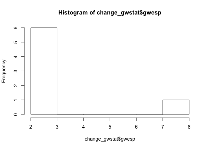
hist(change_gwstat$gwesp) #not very interesting in this simple case
Amazing!
Thanks to Steve Goodreau for help and clarifications.